Inferential statistics¶

Inferential statistics consist in making inferences (generalizations) about the population based on information from sample(s). Simulamath offers you the implementation of hypothesis testing and confidence interval estimation.

The examples in this section comes from the book Elementary Statistics, A step by step approach, 8th Edition, by Professor Allan G. Bluman

How to get to Inferential statistics’ section in Simulamath¶

In the image below is the home page of Simulamath

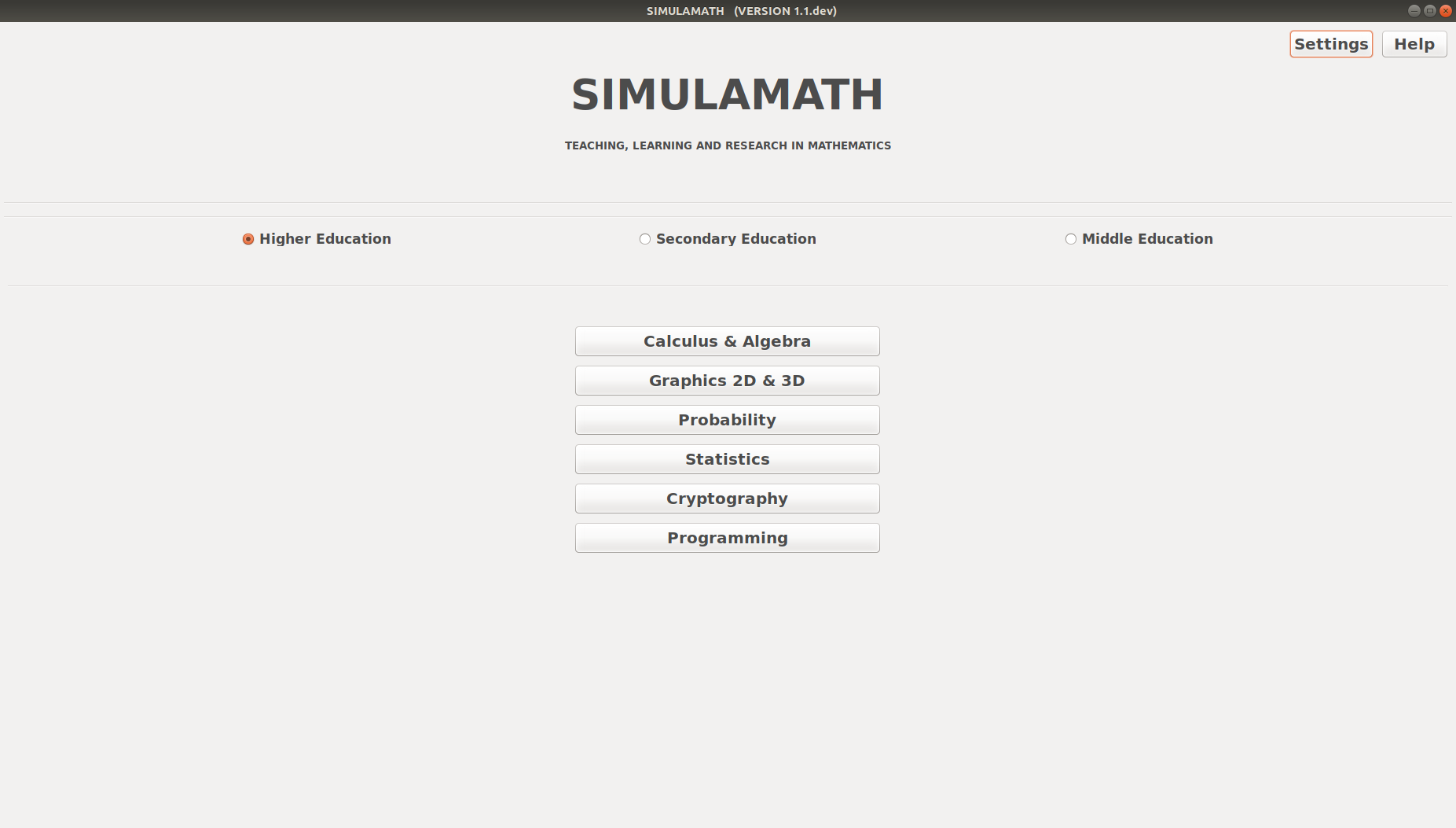
Click on Statistics (just posing the cusor without clicking is also enough)

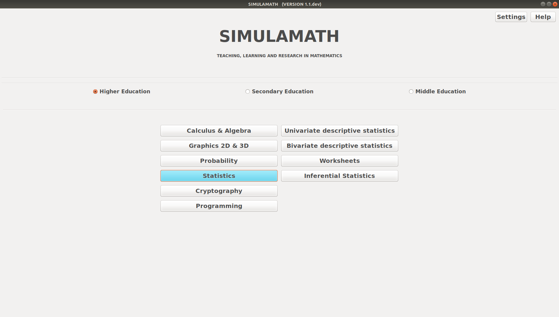
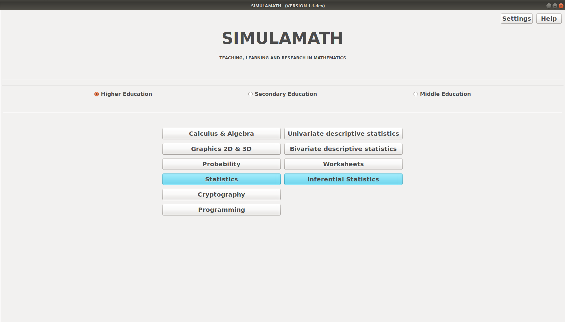
Then you can choose/click your theme of interest, here Inferential Statistics.

Confidence Intervals Estimation¶

Z-Estimation for Mean¶

The formula to get the interval confidence for Z-Estimation for Mean is:

\[\bar{X} - z_{\alpha / 2}\bigg(\dfrac{\sigma}{\sqrt{n}}\bigg) < \mu < \bar{X} + z_{\alpha / 2}\bigg(\dfrac{\sigma}{\sqrt{n}}\bigg)\]

Example:

A survey of 30 emergency room patients found that the average waiting time for treatment was 174.3 minutes. Assuming that the population standard deviation is 46.5 minutes, find the best point estimate of the population mean and the 99% confidence of the population mean.

Solution:

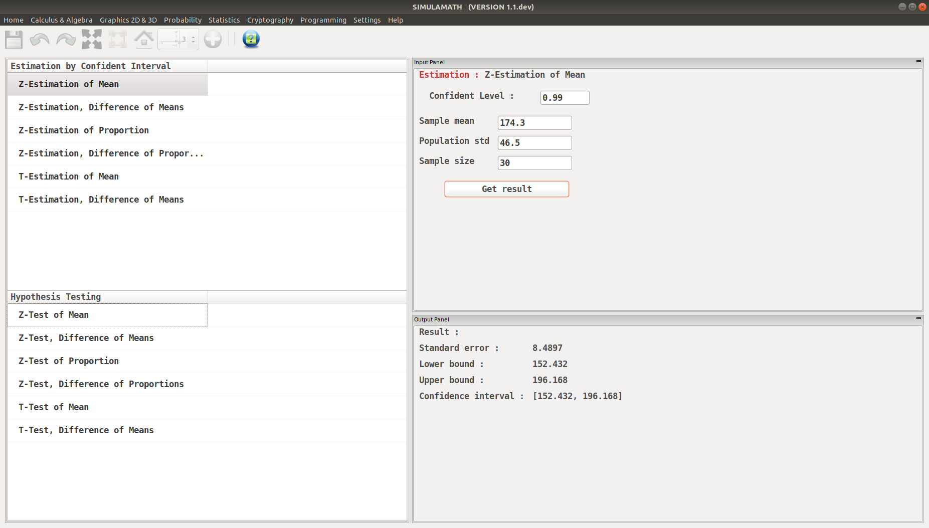
The best point estimate is 174.3 minutes. The 99% confidence is interval is

\[174.3 - 2.58\bigg(\dfrac{46.5}{\sqrt{30}}\bigg) < \mu < 174.3 + 2.58\bigg(\dfrac{46.5}{\sqrt{30}}\bigg)\]

\[152.4 < \mu < 196.2\]

Hence, one can be 99% confident that the mean waiting time for emergency room treatment is between 152.4 and 196.2 minutes.

Z-Estimation for Mean in Simulamath¶

Choose the type of test/estimation you want to compute in the panels on the left hand side, here Z-Estimation for Mean

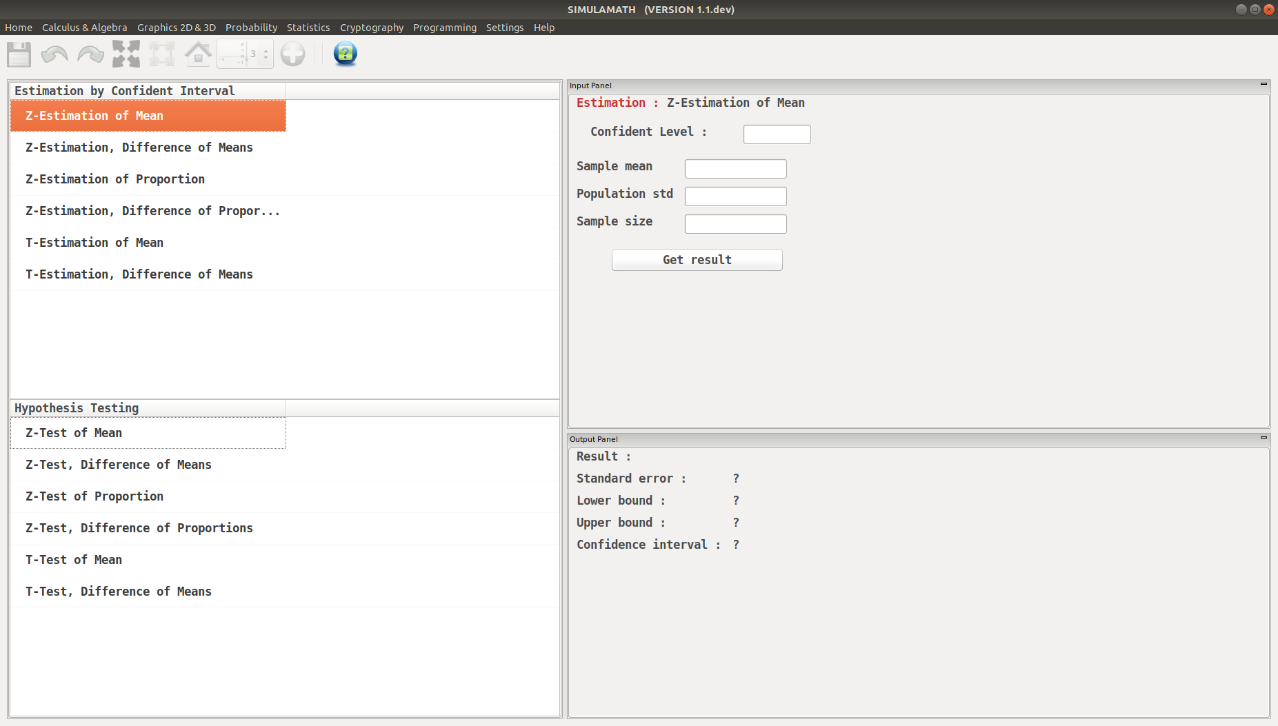
Enter the variables (Confidence level, sample mean, standard deviation of the population, sample size) in the top panel on the right hand side.

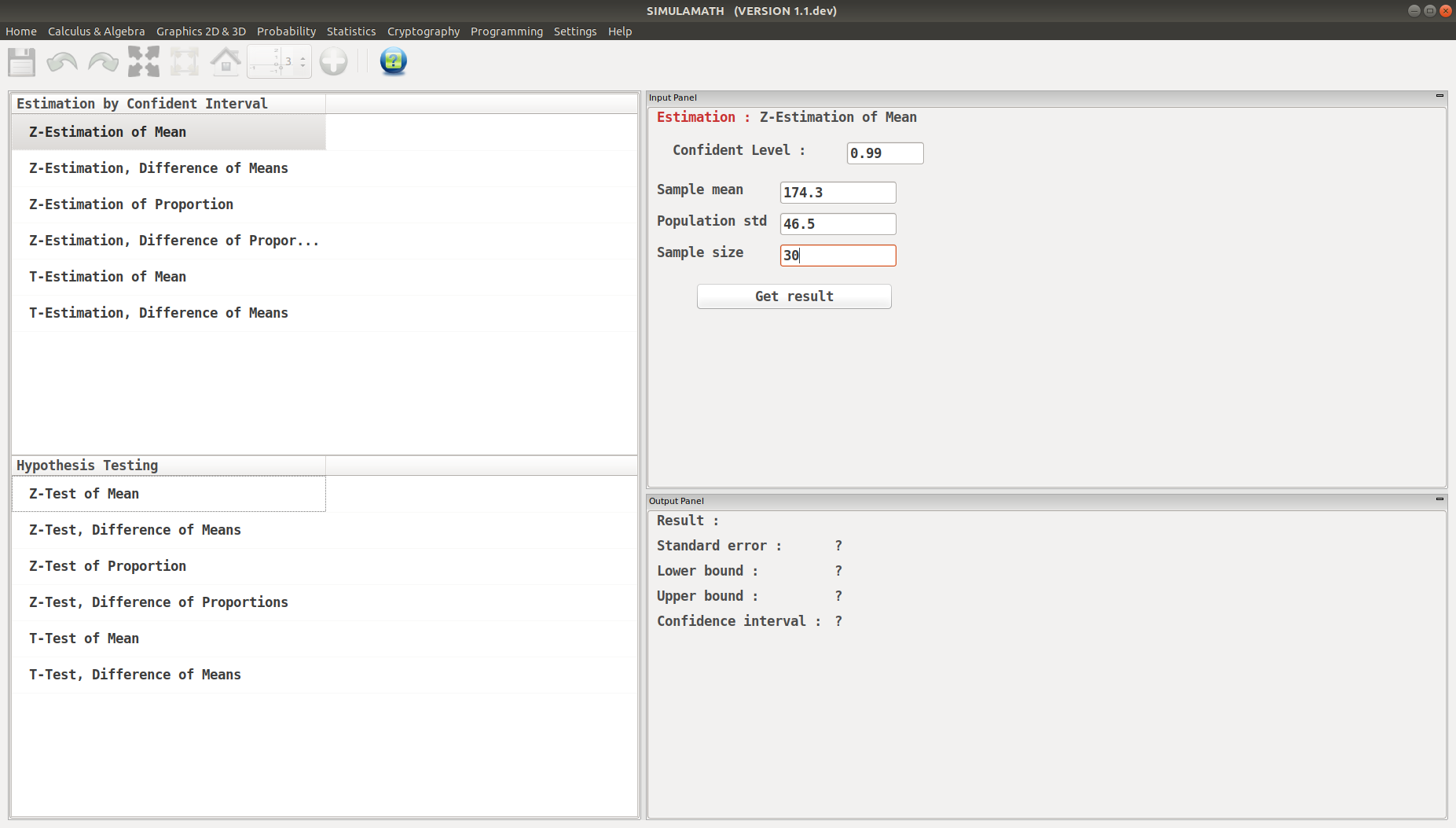
Click on Get result located below inside the same panel. Voila, you have your results in the panel down on the right hand side.

Z-Estimation, Difference of Means¶

The formula to get the interval confidence for Z-Estimation, Difference of Means is:

\[(\bar{X_1} - \bar{X_2}) - z_{\alpha / 2}\sqrt{\dfrac{\sigma_1^2}{n_1}+\dfrac{\sigma_2^2}{n_2}} < \mu_1 - \mu_2 < (\bar{X_1} - \bar{X_2}) + z_{\alpha / 2}\sqrt{\dfrac{\sigma_1^2}{n_1}+\dfrac{\sigma_2^2}{n_2}}\]

Example:

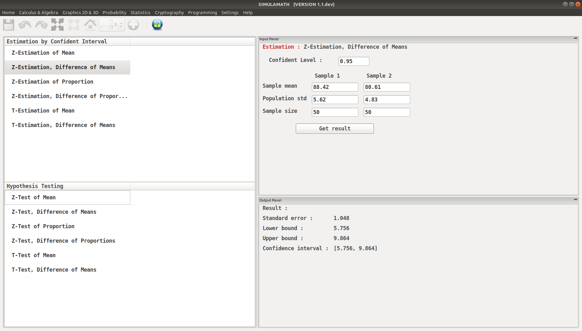
A survey found that the average hotel room rate in New Orleans is $88.42 and the average room rate in Phoenix is $80.61. Assume that the data were obtained from two samples of 50 hotels each and that the standard deviations of the populations are $5.62 and $4.83, respectively. At $\alpha=0.05$, can it be concluded that there is a significant difference in the rates?

Solution:

\[88.42 - 80.61) - 1.96\sqrt{\dfrac{5.62^2}{50}+\dfrac{4.83^2}{50}} < \mu_1 - \mu_2 < (88.42 - 80.61) + 1.96\sqrt{\dfrac{5.62^2}{50}+\dfrac{4.83^2}{50}}\]

\[5.76 < \mu_1 - \mu_2 < 9.86\]

Summarize the results. There is enough evidence to support the claim that the means are not equal. Hence, there is a significant difference in the rates.

Z-Estimation, Difference of Means in Simulamath¶

Choose the type of test/estimation you want to compute in the panels on the left hand side, here Z-Estimation, Difference of Means

Enter the variables (Confidence level, sample mean, standard deviation of the population, sample size) for each sample in the top panel on the right hand side.

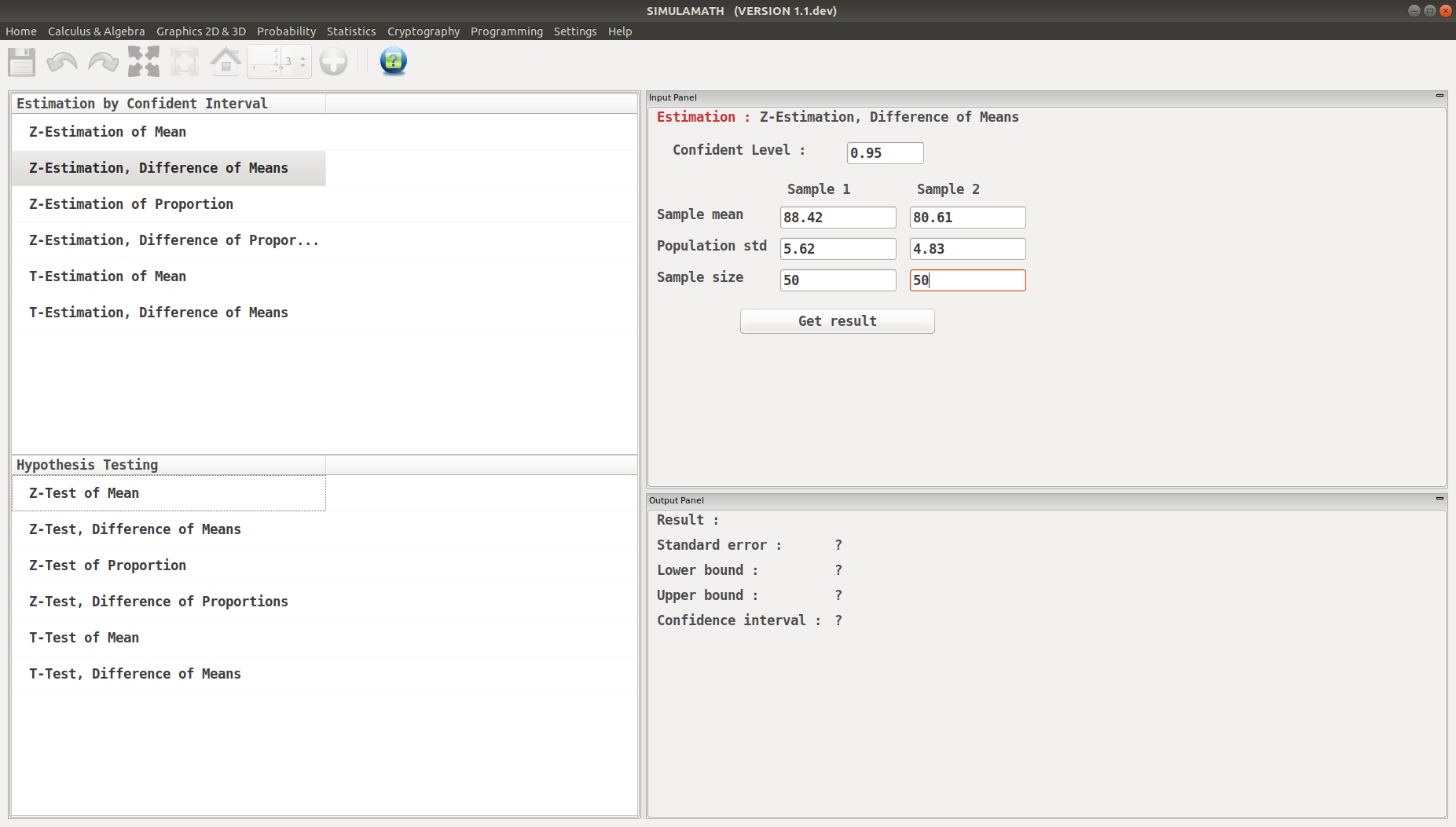
Click on Get result located below inside the same panel. Voila, you have your results in the panel down on the right hand side.

Z-Estimation for Proportion¶

The formula to get the interval confidence for Z-Estimation for Proportion is:

\[\hat{p} - z_{\alpha / 2}\sqrt{\dfrac{\hat{p}\hat{q}}{n}} < p < \hat{p} + z_{\alpha / 2}\sqrt{\dfrac{\hat{p}\hat{q}}{n}}\]

With $\quad \hat{p} = \dfrac{X}{n} \quad \quad \hat{q} = 1 - p$

Assumptions for Testing a Proportion

The sample is a random sample.
The conditions for a binomial experiment are satisfied.
$n_{p} \geq 5$ and $n_{q} \geq 5$.

Example:

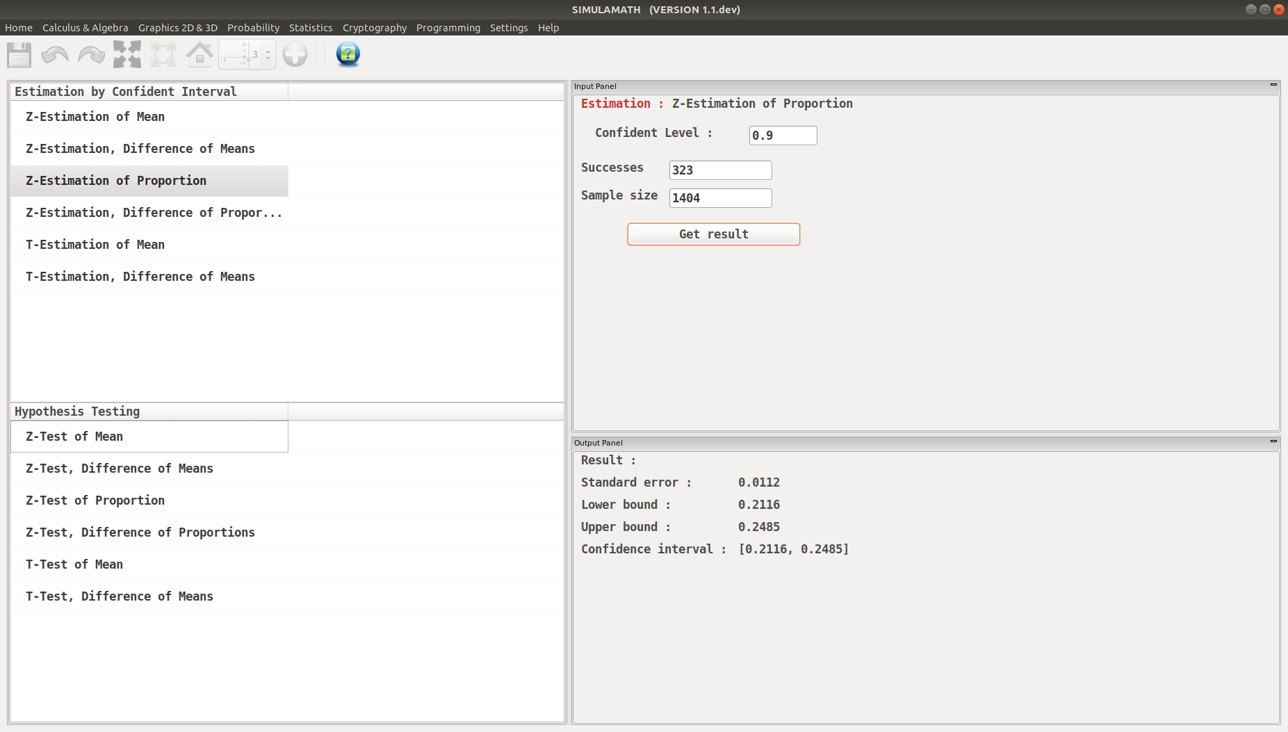
A survey conducted by Sallie Mae and Gallup of 1404 respondents found that 323 students paid for their education by student loans. Find the 90% confidence of the true proportion of students who paid for their education by student loans.

Solution:

Since $\alpha = 1- 0.90 = 0.10$ and $z_{\alpha /2}=1.65$

Replacing it in the above formula we have

\[0.23 - 1.65\sqrt{\dfrac{0.23*0.77}{1404}} < p < 0.23 + \sqrt{\dfrac{0.23*0.77}{1404}},\]

With $\hat{p} = \dfrac{323}{1404} = 0.23$ and $\hat{q} = 1 - p =0.77$

Hence

\[0.211 < p < 0.249\]

Z-Estimation for Proportion in Simulamath¶

Choose the type of test/estimation you want to compute in the panels on the left hand side, here Z-Estimation for Proportion

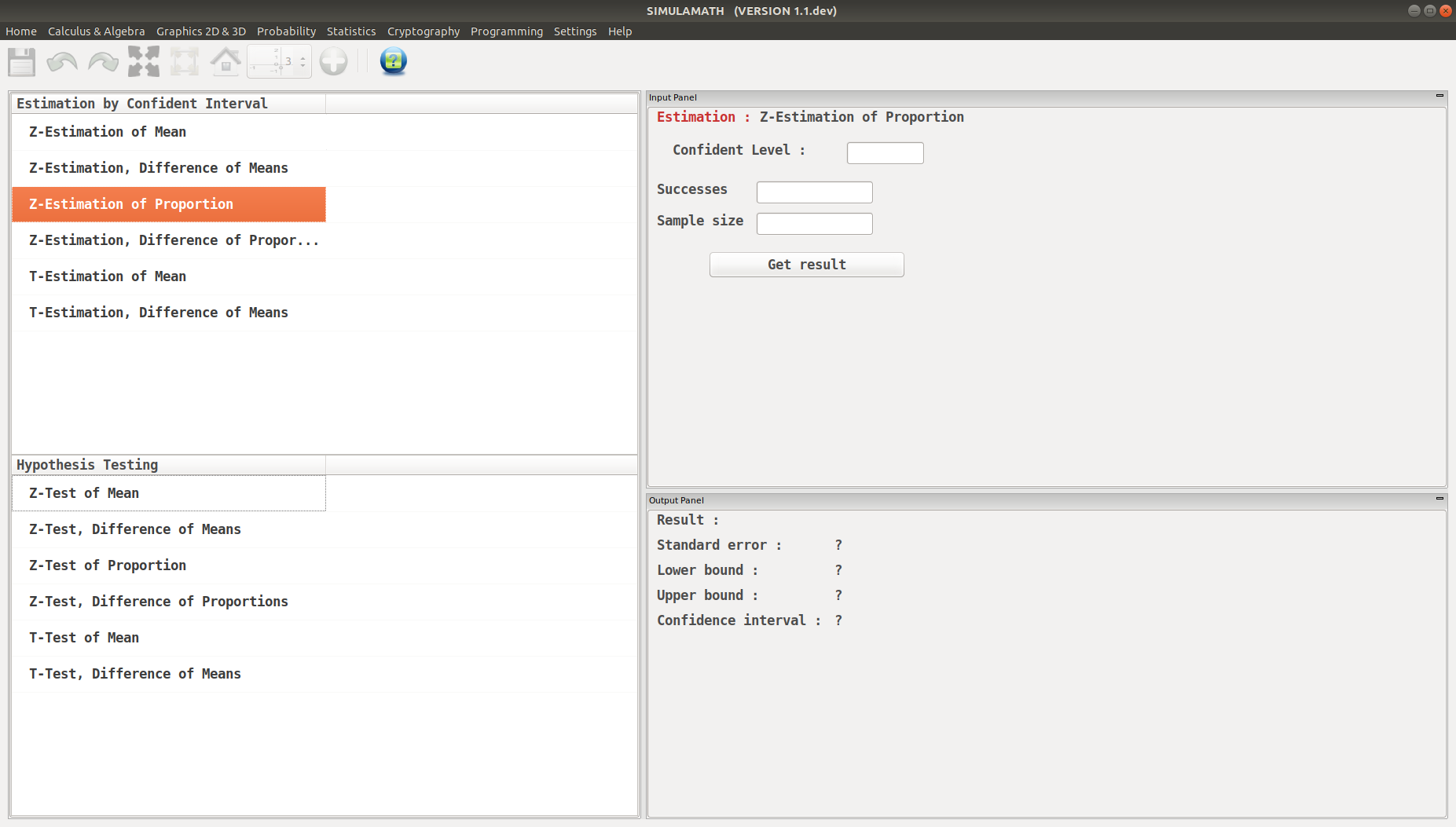
Enter the variables (Confidence level, Success, Sample size) in the top panel on the right hand side.

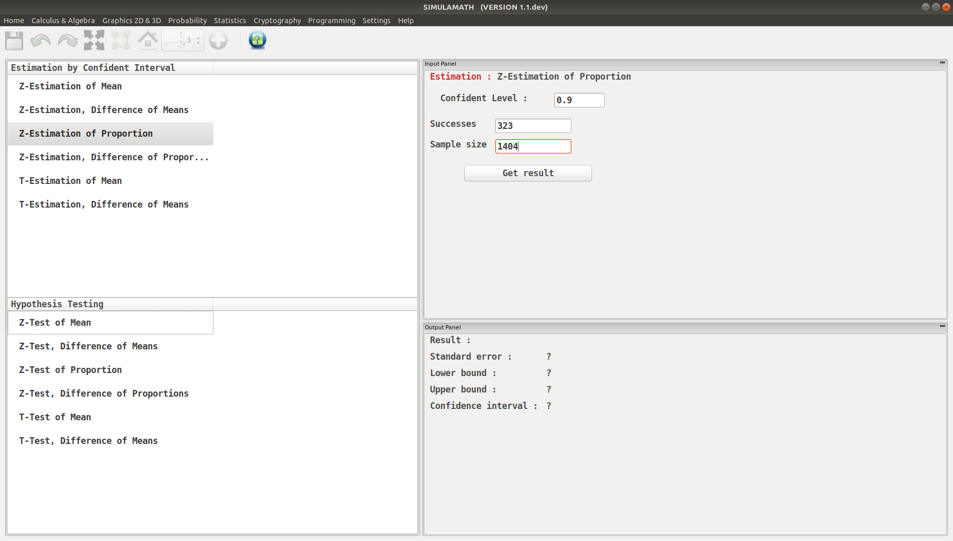
Click on Get result located below inside the same panel. Voila, you have your results in the panel down on the right hand side.

Z-Estimation, Difference of Proportions¶

The formula to get the interval confidence for Z-Estimation, Difference of Proportions is:

\[(\hat{p_1} - \hat{p_2}) - z_{\alpha / 2}\sqrt{\dfrac{\hat{p_1}\hat{q_1}}{n_1}+\dfrac{\hat{p_1}\hat{q_1}}{n_2}} < p_1 - p_2 < (\hat{p_1} - \hat{p_2}) + z_{\alpha / 2}\sqrt{\dfrac{\hat{p_1}\hat{q_1}}{n_1}+\dfrac{\hat{p_1}\hat{q_1}}{n_2}}\]

Example:

Researchers found that 12 out of 34 small nursing homes had a resident vaccination rate of less than 80%, while 17 out of 24 large nursing homes had a vaccination rate of less than 80%. At a $\alpha=0.05$, test the claim that there is no difference in the proportions of the small and large nursing homes with a resident vaccination rate of less than 80%.

Solution:

Replacing in the above formula we get

\[(0.35 - 0.71) - 1.96\sqrt{\dfrac{0.35*0.65}{34}+\dfrac{0.71*0.29}{24}} < p_1 - p_2 < (0.35 - 0.71) + 1.96\sqrt{\dfrac{0.35*0.65}{34}+\dfrac{0.71*0.29}{24}}\]

\[-0.602 < p_1 - p_2 < -0.118\]

Since 0 is not contained in the interval, the decision is to reject the null hypothesis $H_0 : p_1 = p_2$ .

Z-Estimation, Difference of Proportions in Simulamath¶

Choose the type of test/estimation you want to compute in the panels on the left hand side, here Z-Estimation, Difference of Proportions

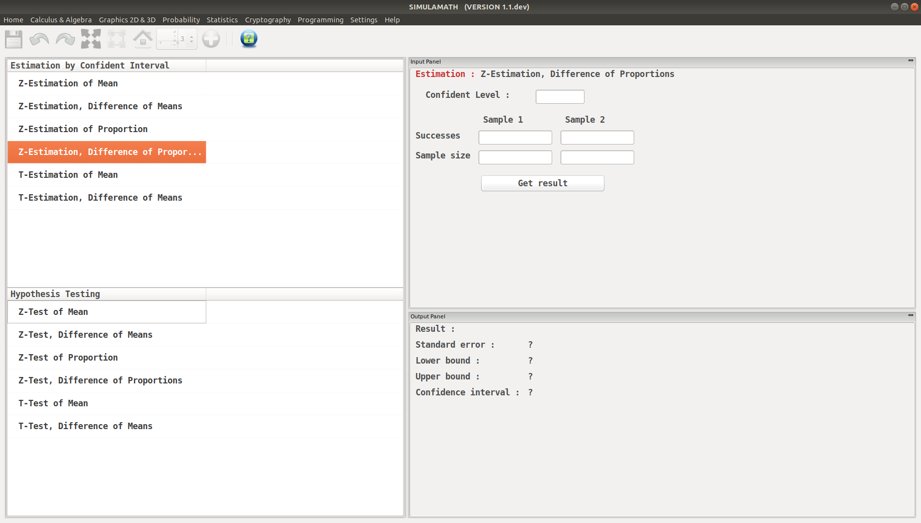
Enter the variables (Confidence level, Success, Sample size) for each sample in the top panel on the right hand side.

Click on Get result located below inside the same panel. Voila, you have your results in the panel down on the right hand side.

T-Estimation for Mean¶

The formula to get the interval confidence for T-Estimation for Mean is:

\[\bar{X} - t_{\alpha / 2}\bigg(\dfrac{s}{\sqrt{n}}\bigg) < \mu < \bar{X} + t_{\alpha / 2}\bigg(\dfrac{s}{\sqrt{n}}\bigg)\]

Assumptions for finding a Confidence interval for a Mean when $\sigma$ is Unknown

The sample is a random sample.
Either $n \geq 30$ or the population is normally distributed if math:n < 30.

Example:

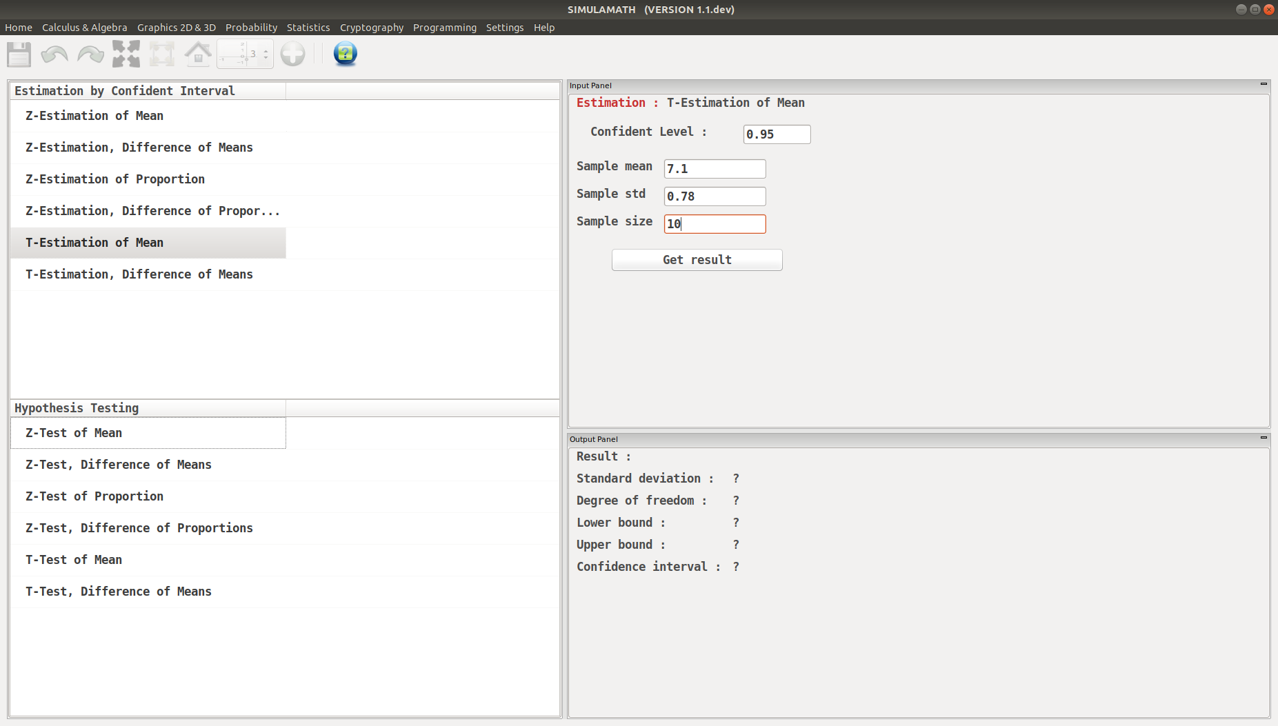
Ten randomly selected people were asked how long they slept at night. The mean time was 7.1 hours, and the standard deviation was 0.78 hour. Find the 95% confidence interval of the mean time. Assume the variable is normally distributed. Solution:

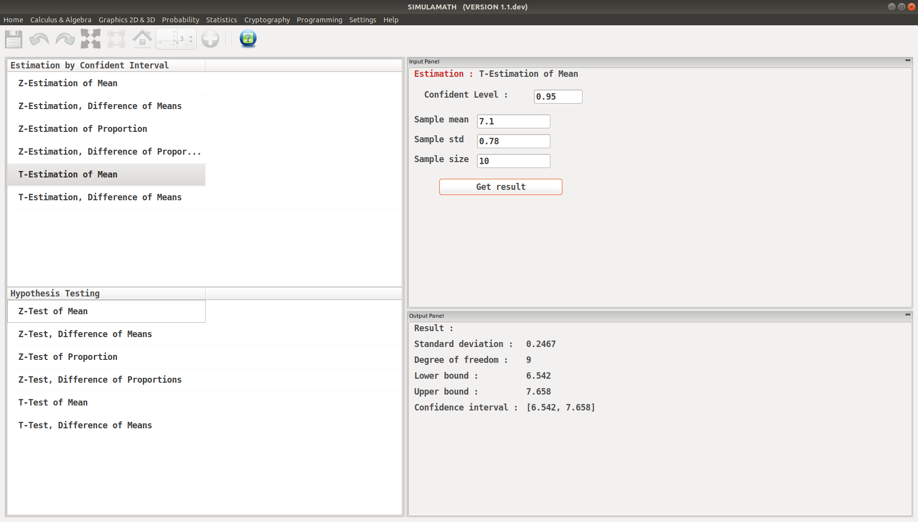
Since $\sigma$ is unknown and $s$ must replace it, the $t$ distribution (Table F) must be used for the confidence interval. Hence, with 9 degrees of freedom $t_{\alpha / 2} = 2.262$. The 95% confidence interval can be found by substituting in the above formula.

\[7.1 - 2.262\bigg(\dfrac{0.78}{\sqrt{10}}\bigg) < \mu < 7.1 + 2.262\bigg(\dfrac{0.78}{\sqrt{10}}\bigg)\]

\[6.54 < \mu < 7.66\]

Therefore, one can be 95% confident that the population mean is between 6.54 and 7.66 hours.

T-Estimation for Mean in Simulamath¶

Choose the type of test/estimation you want to compute in the panels on the left hand side, here T-Estimation for Mean

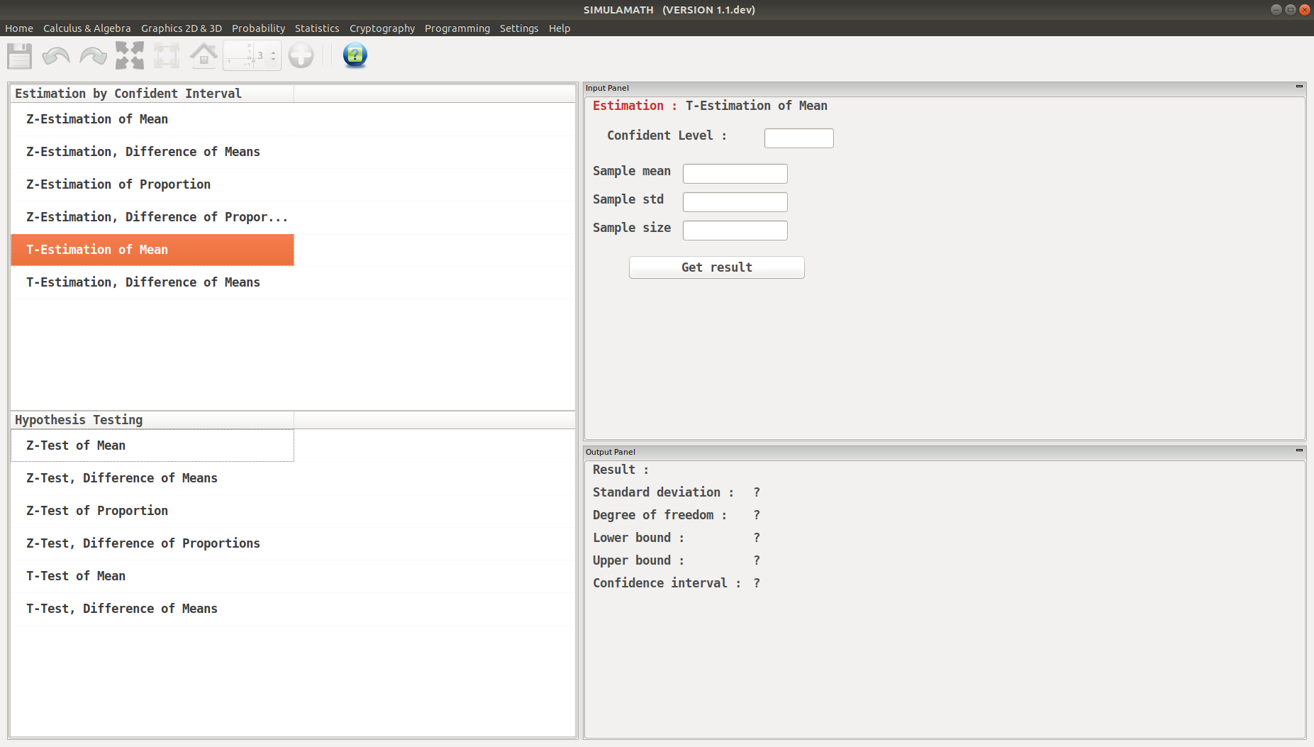
Enter the variables (Confidence level, sample mean, standard deviation of the sample, sample size) in the top panel on the right hand side.

Click on Get result located below inside the same panel. Voila, you have your results in the panel down on the right hand side.

T-Estimation, Difference of Means¶

The formula to get the interval confidence for T-Estimation, Difference of Means is:

\[(\bar{X_1} - \bar{X_2}) - t_{\alpha / 2}\sqrt{\dfrac{s_1^2}{n_1}+\dfrac{s_2^2}{n_2}} < \mu_1 - \mu_2 < (\bar{X_1} - \bar{X_2}) + t_{\alpha / 2}\sqrt{\dfrac{s_1^2}{n_1}+\dfrac{s_2^2}{n_2}}\]

Example:

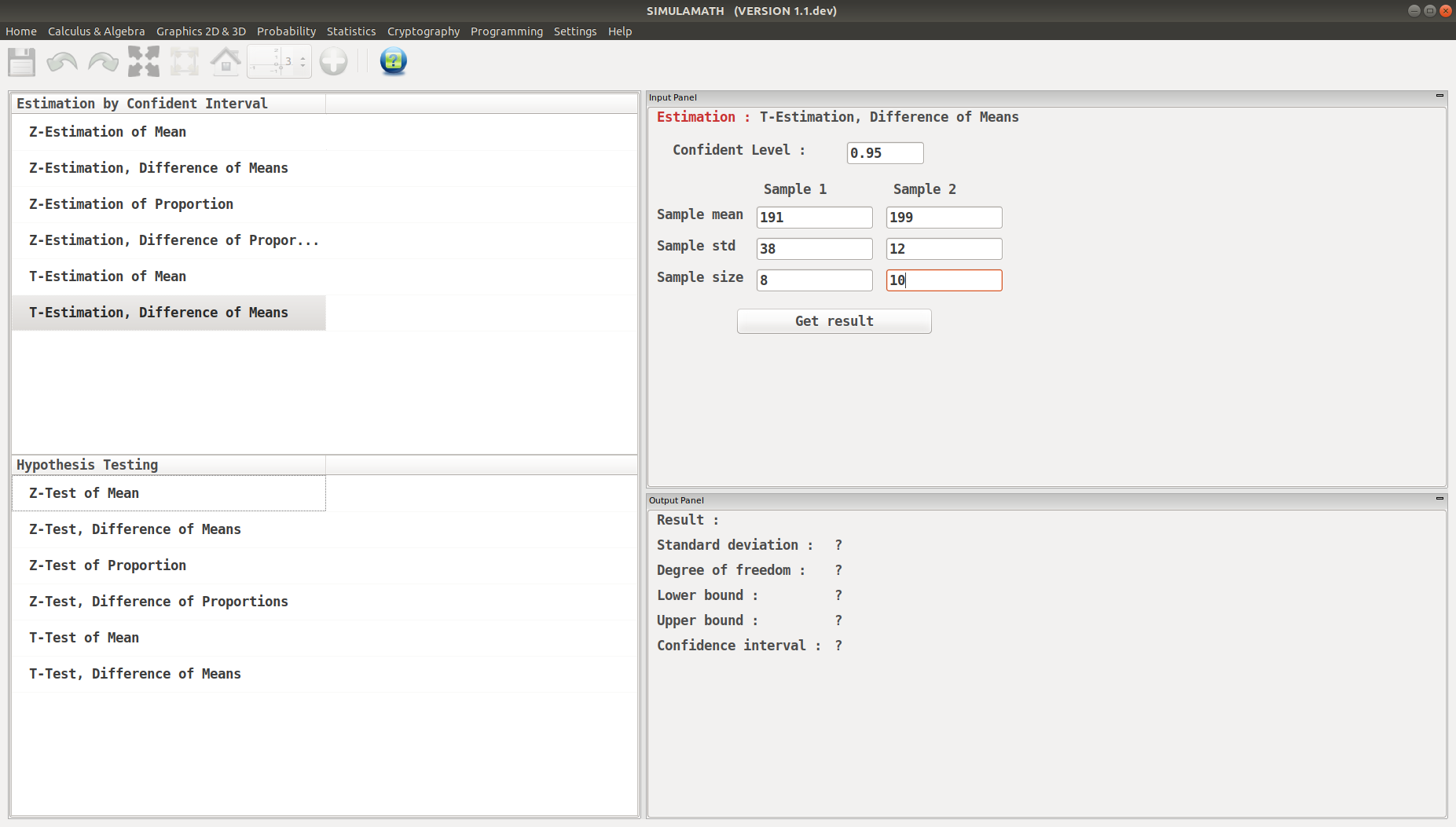
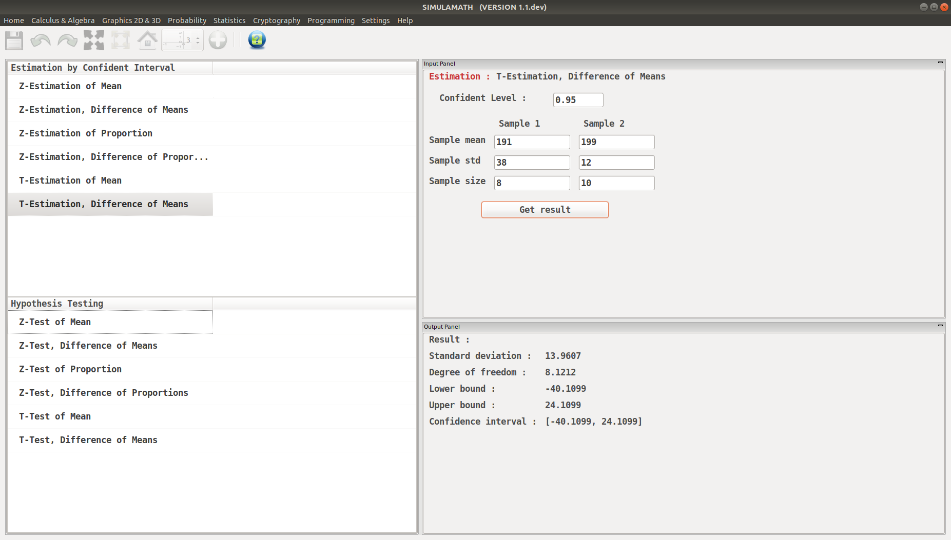
The average size of a farm in Indiana County, Pennsylvania, is 191 acres. The average size of a farm in Greene County, Pennsylvania, is 199 acres. Assume the data were obtained from two samples with standard deviations of 38 and 12 acres, respectively, and sample sizes of 8 and 10, respectively. Can it be concluded at a $\alpha=0.05$ that the average size of the farms in the two counties is different? Assume the populations are normally distributed. Solution:

Replacing in the above formula

\[(191 - 199) - 2.365\sqrt{\dfrac{38^2}{8}+\dfrac{12^2}{10}} < \mu_1 - \mu_2 < (191 - 199) + 2.365\sqrt{\dfrac{38^2}{8}+\dfrac{12^2}{10}}\]

\[-41.02 < \mu_1 - \mu_2 < 25.02\]

Since 0 is contained in the interval, the decision is to not reject the null hypothesis $H_0 : \mu_1 = \mu_2$.

T-Estimation, Difference of Means in Simulamath¶

Choose the type of test/estimation you want to compute in the panels on the left hand side, here T-Estimation, Difference of Means

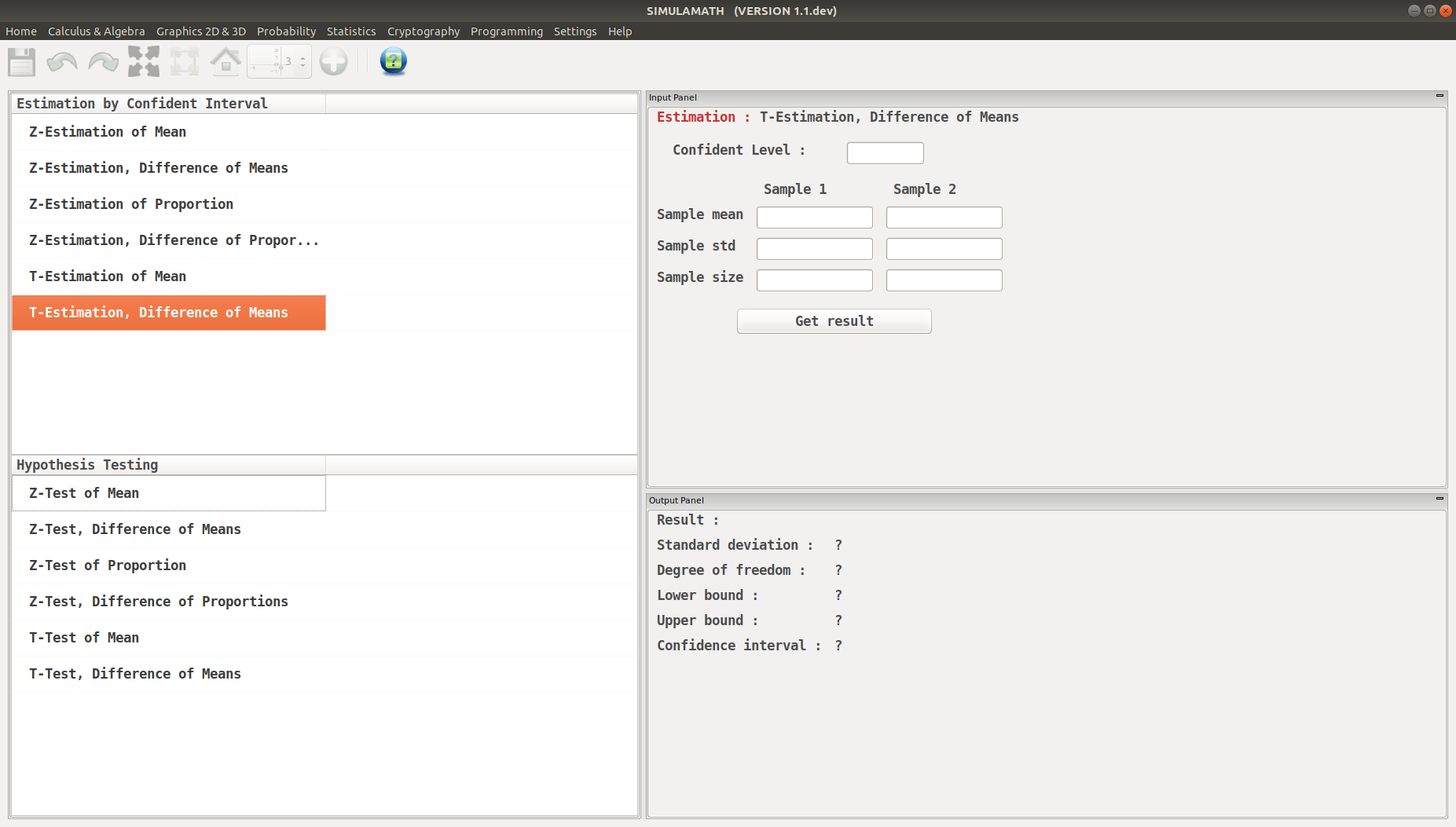
Enter the variables (Confidence level, sample mean, standard deviation of the sample, sample size) for each sample in the top panel on the right hand side.

Click on Get result located below inside the same panel. Voila, you have your results in the panel down on the right hand side.

Hypothesis Testing¶

Z-Test for a Mean¶

The formula for hypothesis testing for Z-Test for a Mean is:

\[z = \dfrac{\bar{X} - \mu}{\frac{\sigma}{\sqrt{n}}}\]

Assumptions for the z-Test for a Mean when $\sigma$ is known

The sample is a random sample.
Either $n \geq30$ or the population is normally distributed if $n < 30$.

Example:

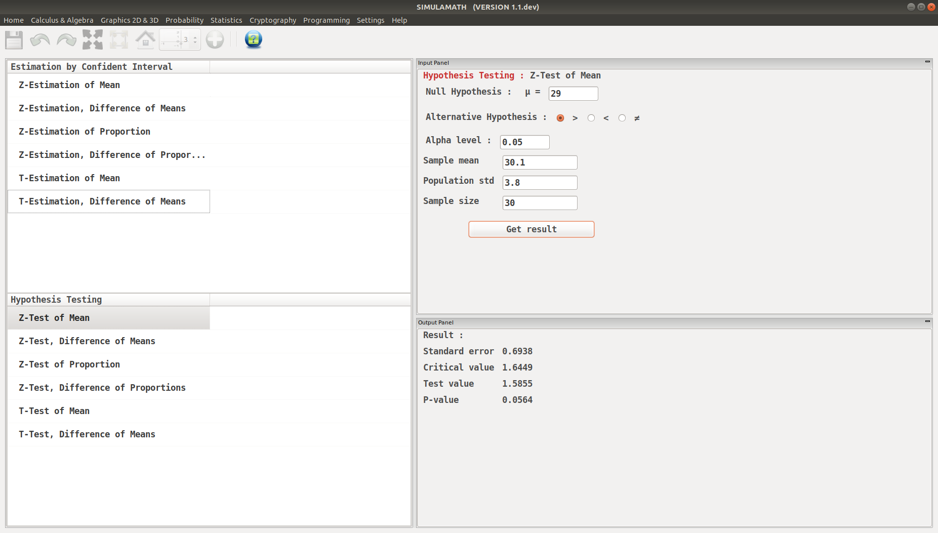
A researcher wishes to see if the mean number of days that a basic, low-price, small automobile sits on a dealer’s lot is 29. A sample of 30 automobile dealers has a mean of 30.1 days for basic, low-price, small automobiles. At $\alpha=0.05$, test the claim that the mean time is greater than 29 days. The standard deviation of the population is 3.8 days.

Solution:

Step 1: State the hypotheses and identify the claim.

\[H_0: \mu = 29 \quad \text{and} \quad H_1: \mu > 29 \text{(claim)}\]

Step 2: Find the critical value. Since $\alpha=0.05$ and the test is a right-tailed test, the critical value is $z = +1.65$.

Step 3: Compute the test value.

\[z = \dfrac{\bar{X} - \mu}{\frac{\sigma}{\sqrt{n}}}\]

\[z = \dfrac{30.1 - 29}{\frac{3.8}{\sqrt{3}}} = 1.59\]

Step 4: Make the decision. Since the test value, +1.59, is less than the critical value, +1.65, and is not in the critical region, the decision is to not reject the null hypothesis.

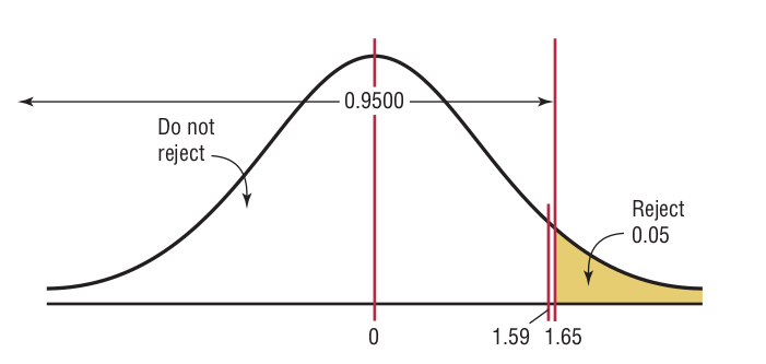
Step 5: Summarize the results. There is not enough evidence to support the claim that the mean time is greater than 29 days.

Z-Test for a Mean in Simulamath¶

Choose the type of test/estimation you want to compute in the panels on the left hand side, here Z-Estimation of Mean

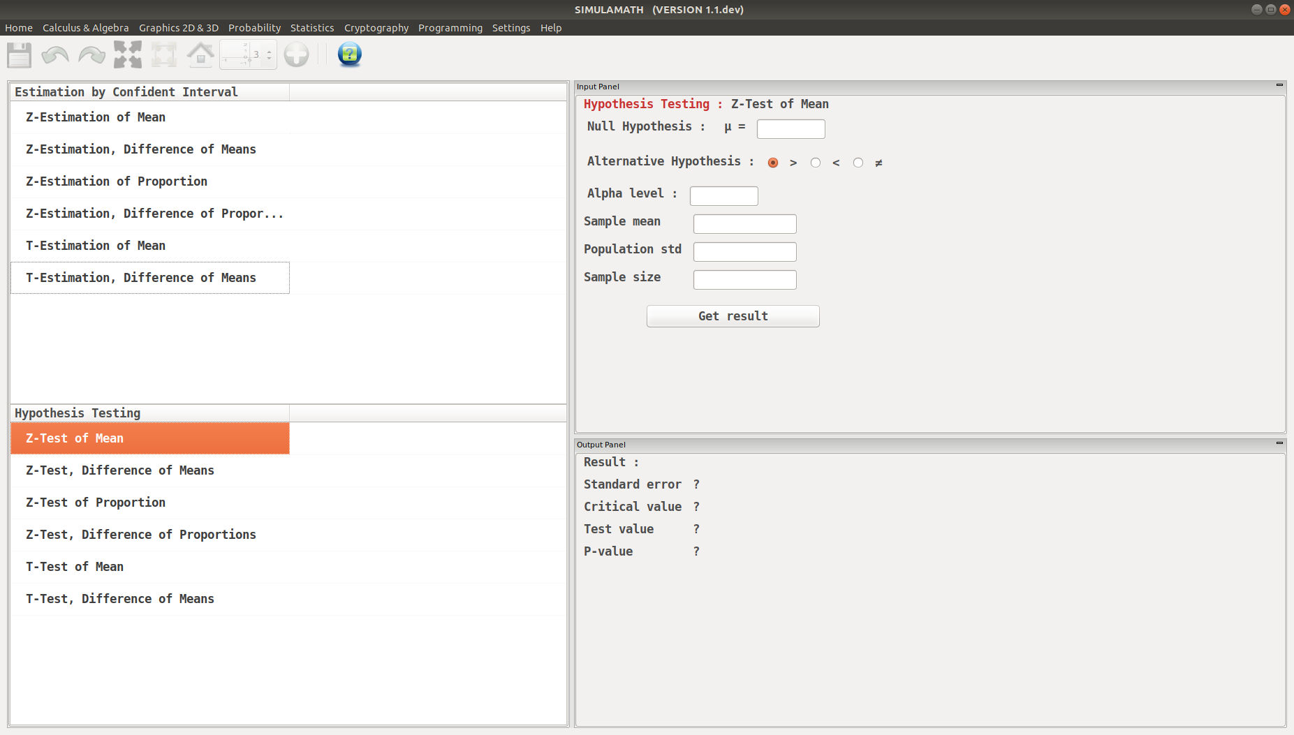
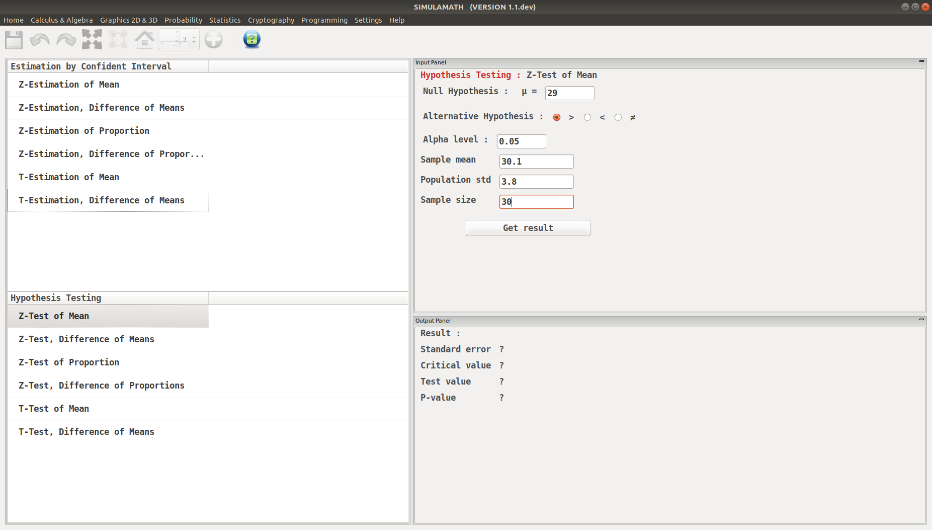
Enter the variables (Null Hypothesis, Alternative Hypothesis, Alpha value, Sample mean, Population standard deviation, Sample size) in the top panel on the right hand side.

Click on Get result located below inside the same panel. Voila, you have your results in the panel down on the right hand side.

Z-Test, Difference of Means¶

The formula for hypothesis testing for Z-Test, Difference of Means is:

\[z = \dfrac{(\bar{X_1}-\bar{X_2}) - (\mu_1-\mu_1)}{\sqrt{\dfrac{\sigma_1^2}{n_1} + \dfrac{\sigma_2^2}{n_2} }}\]

\[\text{Test value} = \dfrac{(\text{observed value)} - (\text{expected value})} {\text{standard error}}\]

Example:

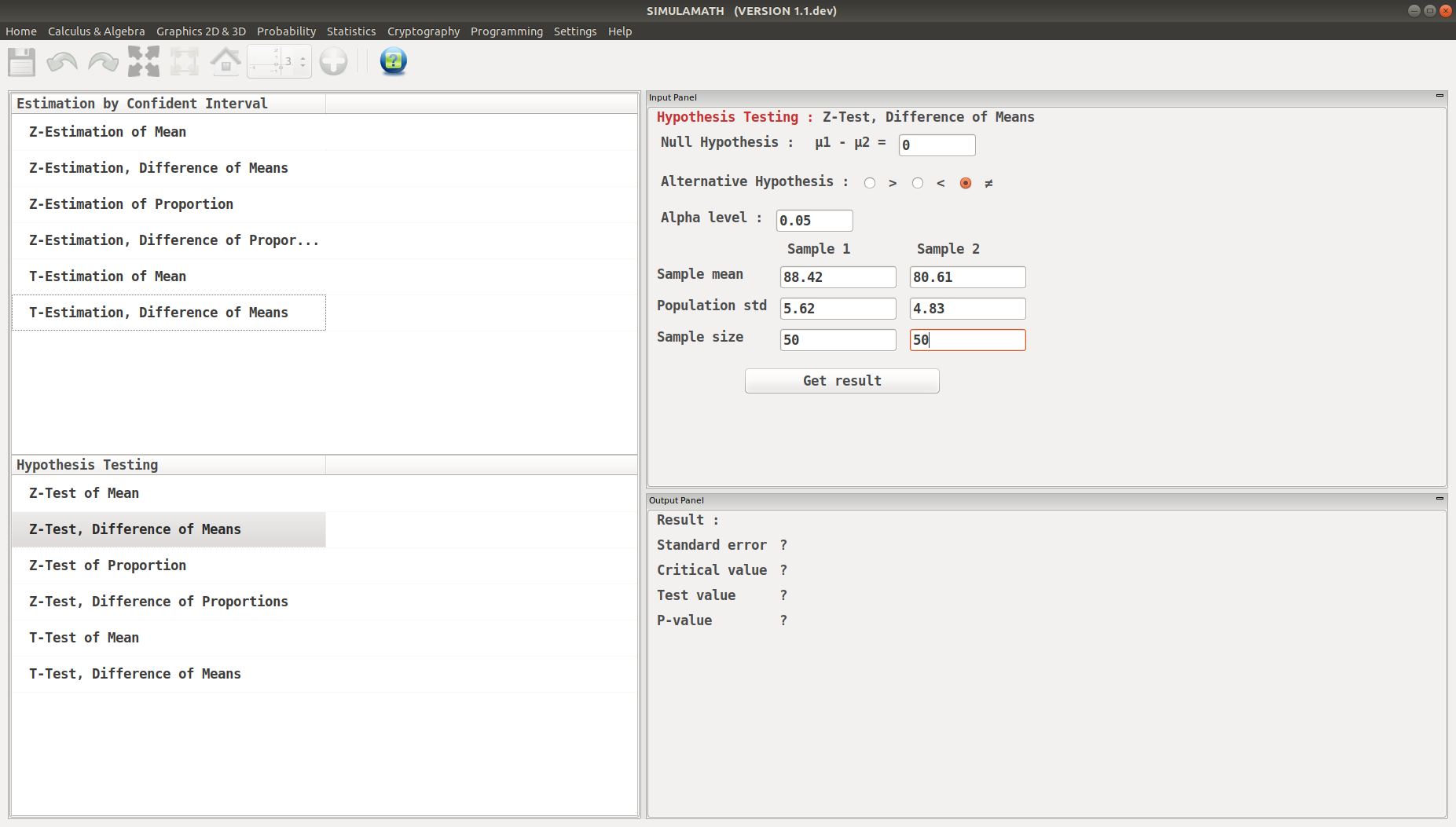
A survey found that the average hotel room rate in New Orleans is $88.42 and the average room rate in Phoenix is $80.61. Assume that the data were obtained from two samples of 50 hotels each and that the standard deviations of the populations are $5.62 and $4.83, respectively. At $\alpha=0.05$, can it be concluded that there is a significant difference in the rates?

Solution:

Step 1: State the hypotheses and identify the claim.

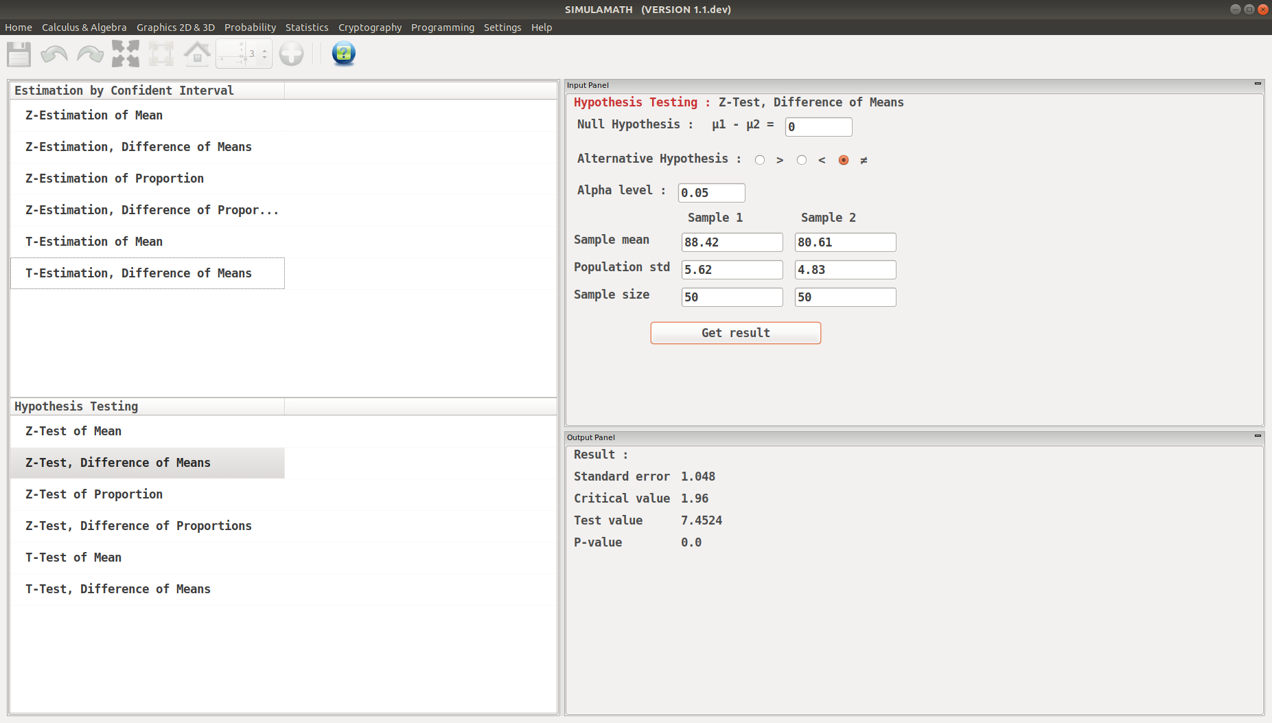
\[H_0: \mu_1 = \mu_2 \quad \text{and} \quad H_1: \mu_1 \neq \mu_2 \text{(claim)}\]

Step 2: Find the critical values. Since $\alpha=0.05$, the critical values are +1.96 and -1.96.

Step 3: Compute the test value.

\[z = \dfrac{(\bar{X_1}-\bar{X_2}) - (\mu_1-\mu_1)}{\sqrt{\dfrac{\sigma_1^2}{n_1} + \dfrac{\sigma_2^2}{n_2} }}\]

\[z = \dfrac{(88.42 - 80.61) - 0}{\sqrt{\dfrac{5.62^2}{50} + \dfrac{4.83^2}{50} }} = 7.45\]

Step 4: Make the decision. Reject the null hypothesis at $\alpha=0.05$, since 7.45 > 1.96.

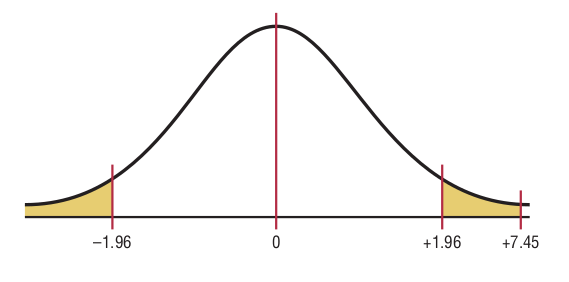
Step 5: Summarize the results. There is enough evidence to support the claim that the means are not equal. Hence, there is a significant difference in the rates.

Z-Test, Difference of Means in Simulamath¶

Choose the type of test/estimation you want to compute in the panels on the left hand side, here Z-Estimation, Difference of Means

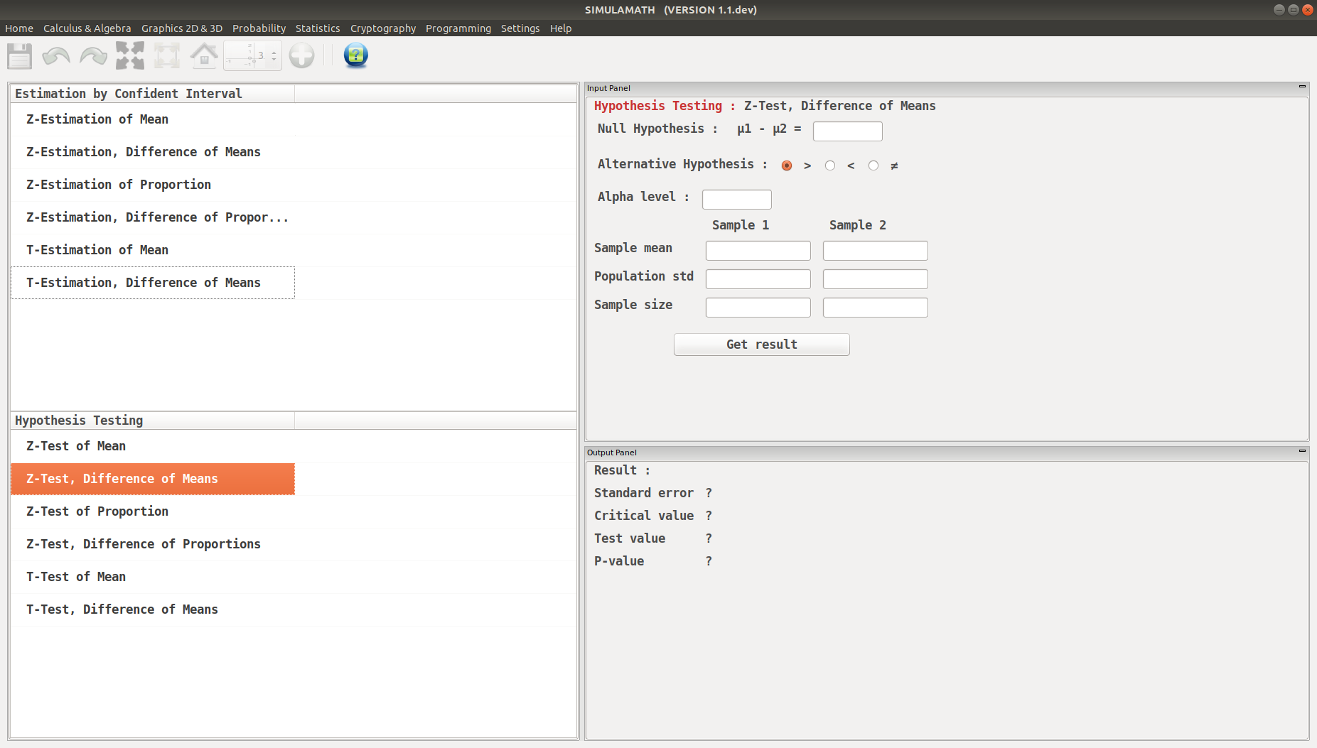
Enter the variables (Null Hypothesis, Alternative Hypothesis, Alpha value, Sample mean, Population standard deviation, Sample size) for each sample in the top panel on the right hand side.

Click on Get result located below inside the same panel. Voila, you have your results in the panel down on the right hand side.

Z-Test for Proportion¶

The formula for hypothesis testing for Z-Test for Proportion is:

\[z = \dfrac{\hat{p} - p}{\sqrt{pq/n}}\]

Assumptions for Testing a Proportion

The sample is a random sample.
The conditions for a binomial experiment are satisfied.
$np \geq 5$ and $nq \geq 5$.

Example:

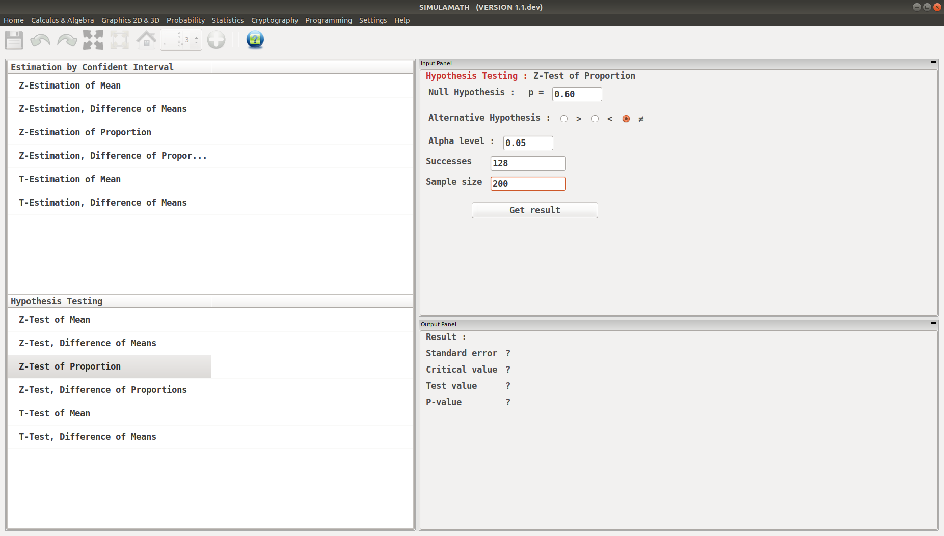
A dietitian claims that 60% of people are trying to avoid trans fats in their diets. She randomly selected 200 people and found that 128 people stated that they were trying to avoid trans fats in their diets. At $\alpha=0.05$, is there enough evidence to reject the dietitian’s claim?

Solution:

Step 1: State the hypothesis and identify the claim.

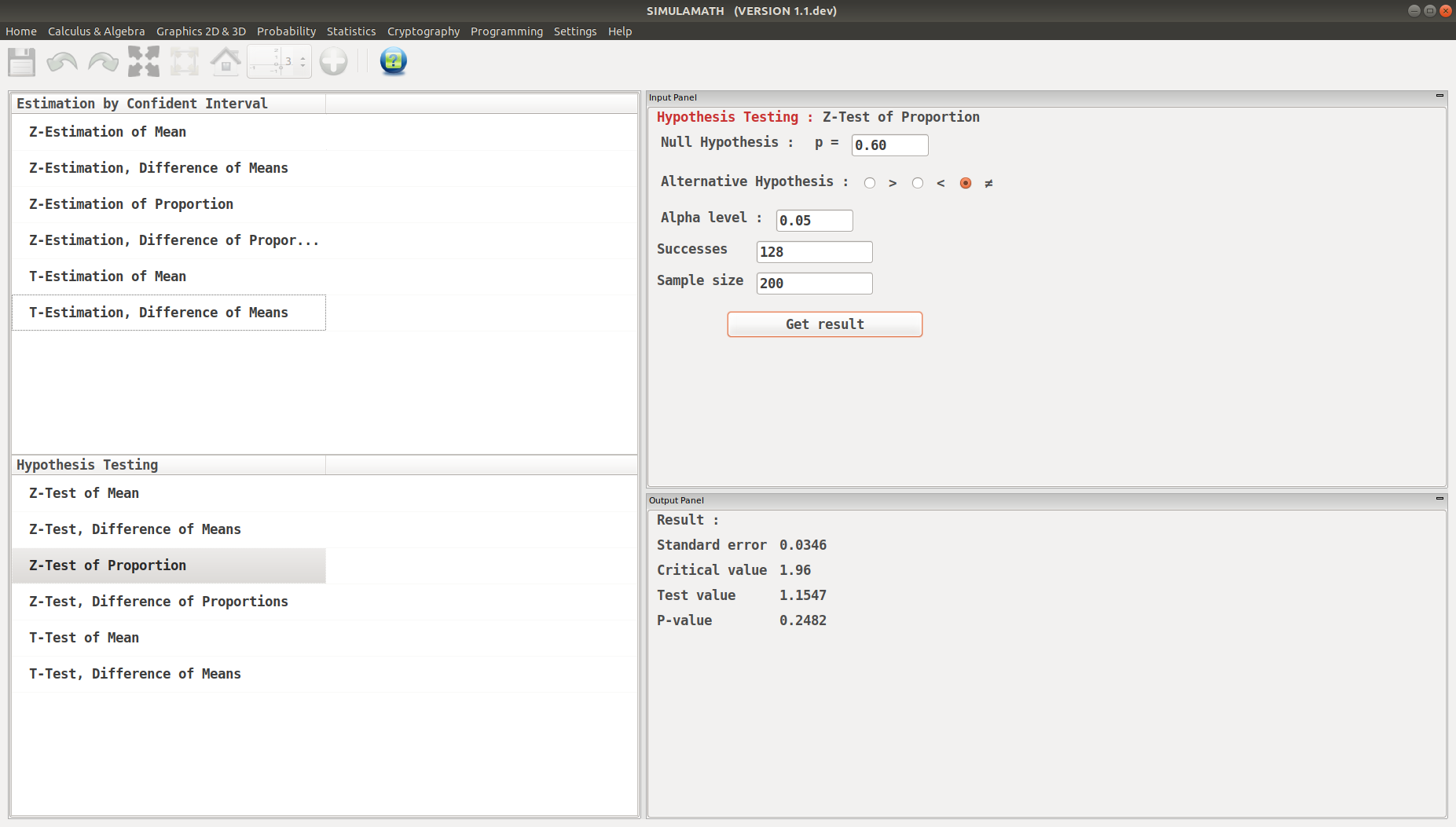
\[H_0: p = 0.60 \quad \text{(claim)} \quad \text{et} \quad H_1: p \neq 0.60\]

Step 2: Find the critical values. Since $\alpha=0.05$ and the test value is two-tailed, the critical values are +1.96 and -1.96.

Step 3: Compute the test value. First, it is necessary to find $\hat{p}$.

\[\hat{p} = \dfrac{X}{n} = \dfrac{128}{200}=0.64 \quad \quad p = 0.60 \quad \text{and then} \quad q = 1-p = 0.40\]

Therefore

\[z = \dfrac{0.64 - 0.60}{\sqrt{ 0.60*0.40/200}} = 1.15\]

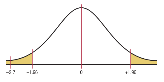
Step 4: Make the decision. Do not reject the null hypothesis since the test value falls outside the critical region, as shown in the figure below

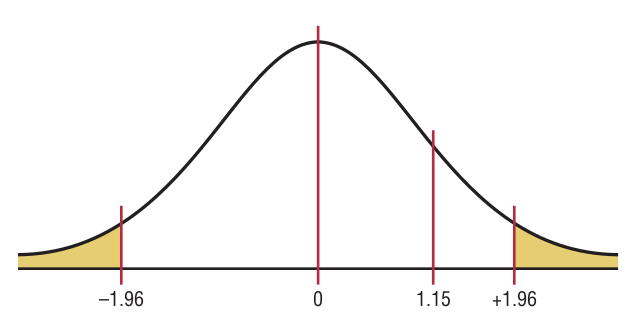
Step 5: Summarize the results. There is not enough evidence to reject the claim that 60% of people are trying to avoid trans fats in their diets.

Z-Test for Proportion in Simulamath¶

Choose the type of test/estimation you want to compute in the panels on the left hand side, here Z-Test for Proportion

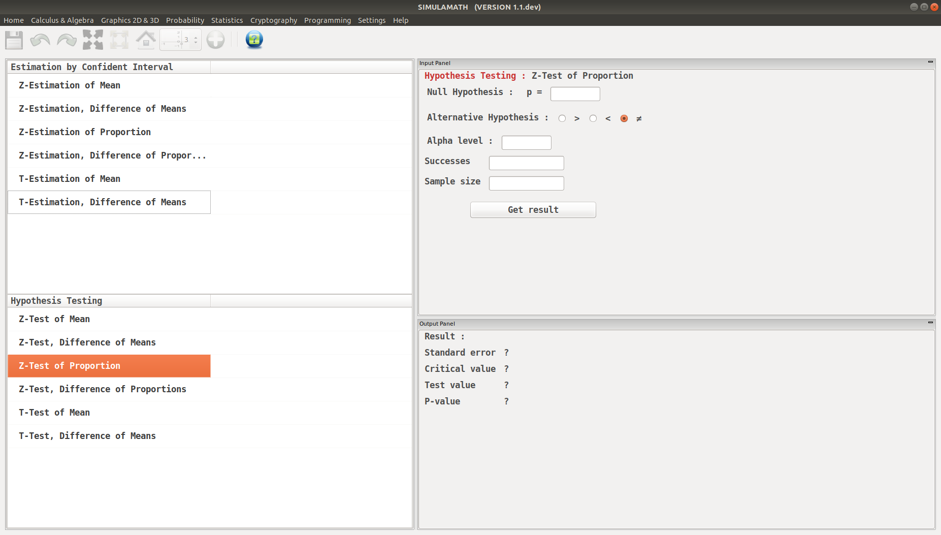
Enter the variables (Null Hypothesis, Alternative Hypothesis, Alpha value, Success, Sample size) in the top panel on the right hand side.

Click on Get result located below inside the same panel. Voila, you have your results in the panel down on the right hand side.

Z-Test, Difference of Proportions¶

The formula for hypothesis testing for Z-Test, Difference of Proportions is:

\[z = \dfrac{(\hat{p_1}-\hat{p_2}) - (p_1-p_1)}{\sqrt{\bar{p}\bar{q}(\dfrac{1}{n_1} + \dfrac{1}{n_2}) }}\]

where

\[\bar{p} = \dfrac{X_1 + X_2}{n_1 + n_2} \quad \quad \hat{p_1} = \dfrac{X_1}{n_1}\]

and

\[\bar{q} = 1 - \bar{p} \quad \quad \hat{p_2} = \dfrac{X_2}{n_2}\]

This formula is based on the general format of

\[\text{Test value} = \dfrac{(\text{observed value)} - (\text{expected value})} {\text{standard error}}\]

Assumptions for the z-Test for Two Proportions

The samples must be random samples.
The sample data are independent of one another.
For both samples $np \geq 5$ and $nq \geq 5$.

Example:

Researchers found that 12 out of 34 small nursing homes had a resident vaccination rate of less than 80%, while 17 out of 24 large nursing homes had a vaccination rate of less than 80%. At $\alpha=0.05$, test the claim that there is no difference in the proportions of the small and large nursing homes with a resident vaccination rate of less than 80%.

Solution:

Let $\hat{p_1}$ be the proportion of the small nursing homes with a vaccination rate of less than 80% and $\hat{p_2}$ be the proportion of the large nursing homes with a vaccination rate of less than 80%. Then

\[\bar{p} = \dfrac{X_1 + X_2}{n_1 + n_2} = \dfrac{12 + 17}{34 + 24}=0.5 \quad \quad \hat{p_1} = \dfrac{X_1}{n_1} = \dfrac{12}{34} = 0.35\]

\[\bar{q} = 1 - \bar{p} = 1-0.5=0.5 \quad \quad \hat{p_2} = \dfrac{X_2}{n_2} = \dfrac{17}{24} = 0.71\]

Step 1: State the hypotheses and identify the claim.

\[H_0: p_1 = p_2 \quad \text{(claim)} \quad \text{and} \quad H_1: p_1 \neq p_2\]

Step 2: Find the critical values. Since $\alpha=0.05$, the critical values are +1.96 and -1.96.

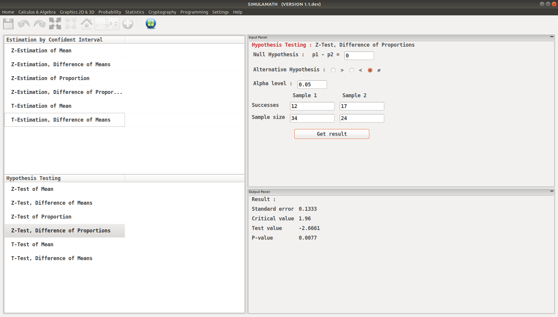
Step 3: Compute the test value.

\[z = \dfrac{(\hat{p_1}-\hat{p_2}) - (p_1-p_1)}{\sqrt{\bar{p}\bar{q}(\dfrac{1}{n_1} + \dfrac{1}{n_2}) }}\]

\[z = \dfrac{(0.35 - 0.75) - 0}{\sqrt{0.5*0.5(\dfrac{1}{34} + \dfrac{1}{24}) }} = -2.7\]

Step 4: Make the decision. Reject the null hypothesis, since -2.7 < -1.96. see figure

Step 5: Summarize the results. There is enough evidence to reject the claim that there is no difference in the proportions of small and large nursing homes with a resident vaccination rate of less than 80%.

Z-Test, Difference of Proportions in Simulamath¶

Choose the type of test/estimation you want to compute in the panels on the left hand side, here Z-Estimation, Difference of Proportions

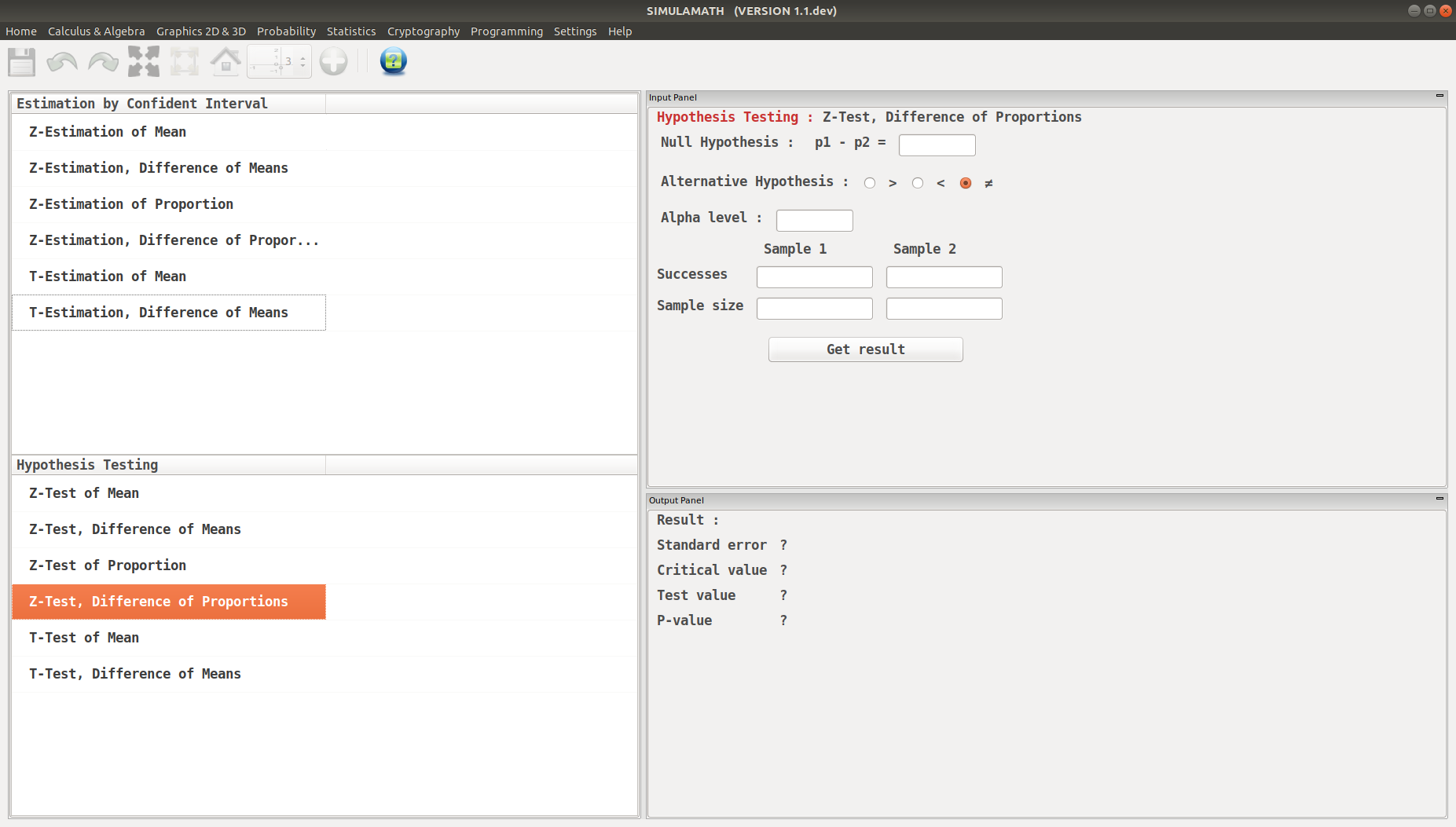
Enter the variables (Null Hypothesis, Alternative Hypothesis, Alpha value, Success, Sample size) for each sample in the top panel on the right hand side.

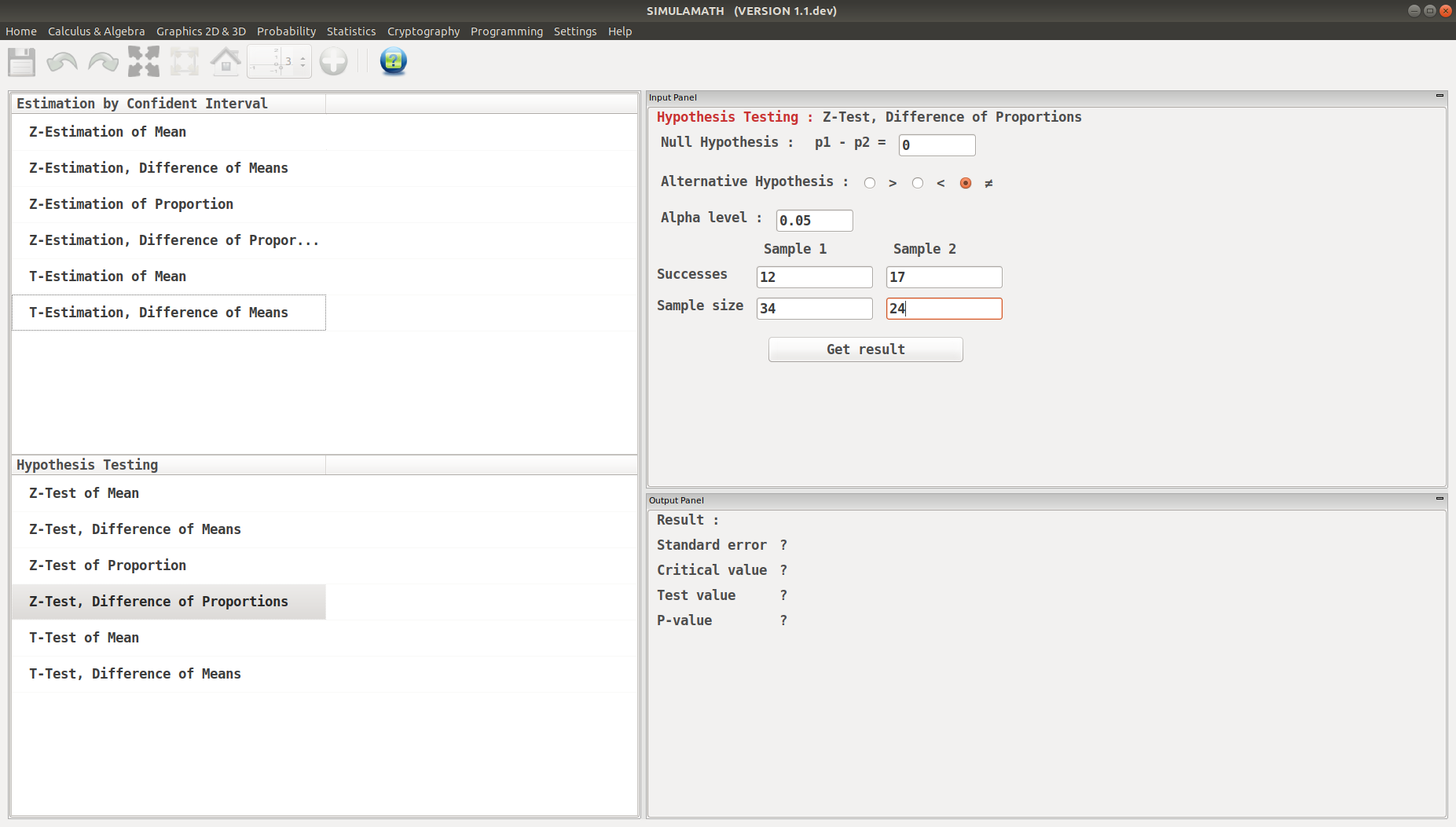
Click on Get result located below inside the same panel. Voila, you have your results in the panel down on the right hand side.

T-Test for a Mean¶

The formula for hypothesis testing for T-Test for a Mean is:

\[t = \dfrac{\bar{X} -\mu}{s/\sqrt{n}}\]

This formula is based on the general format of

\[\text{Test value} = \dfrac{(\text{observed value)} - (\text{expected value})} {\text{standard error}}\]

Assumptions for the t-Test for a Mean When $\sigma$ is unknown

The sample is a random sample.
Either $n \geq 30$ or the population is normally distributed if $n < 30$.

Example:

A medical investigation claims that the average number of infections per week at a hospital in southwestern Pennsylvania is 16.3. A random sample of 10 weeks had a mean number of 17.7 infections. The sample standard deviation is 1.8. Is there enough evidence to reject the investigator’s claim at $\alpha=0.05$? Solution:

Step 1: $H_0: \mu = 16.3 \quad \text{(claim)} \quad \text{and} \quad H_1: \mu \neq 16.3$.

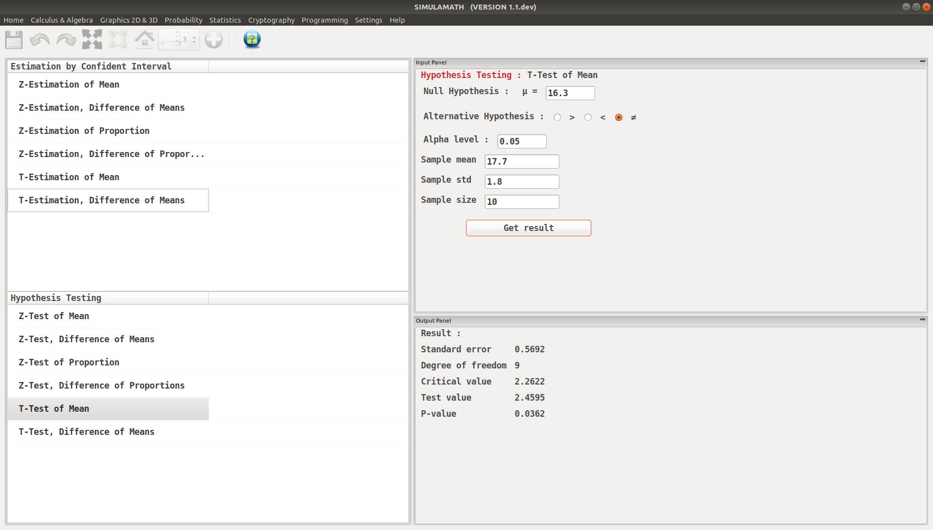
Step 2: The critical values are +2.262 and -2.262 for $\alpha=0,05$ and $d.f= 9$.

Step 3: The test value is

\[t = \dfrac{\bar{X} -\mu}{s/\sqrt{n}} = \dfrac{17.7 -16.3}{1.8/\sqrt{10}} = 2.46\]

Step 4: Reject the null hypothesis since $2.46 > 2.262$.

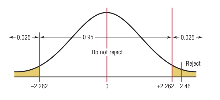
Step 5: There is enough evidence to reject the claim that the average number of infections is 16.3.

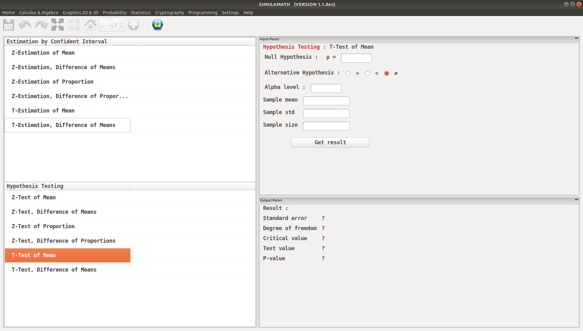
T-Test for a Mean in Simulamath¶

Choose the type of test/estimation you want to compute in the panels on the left hand side, here T-Estimation of Mean

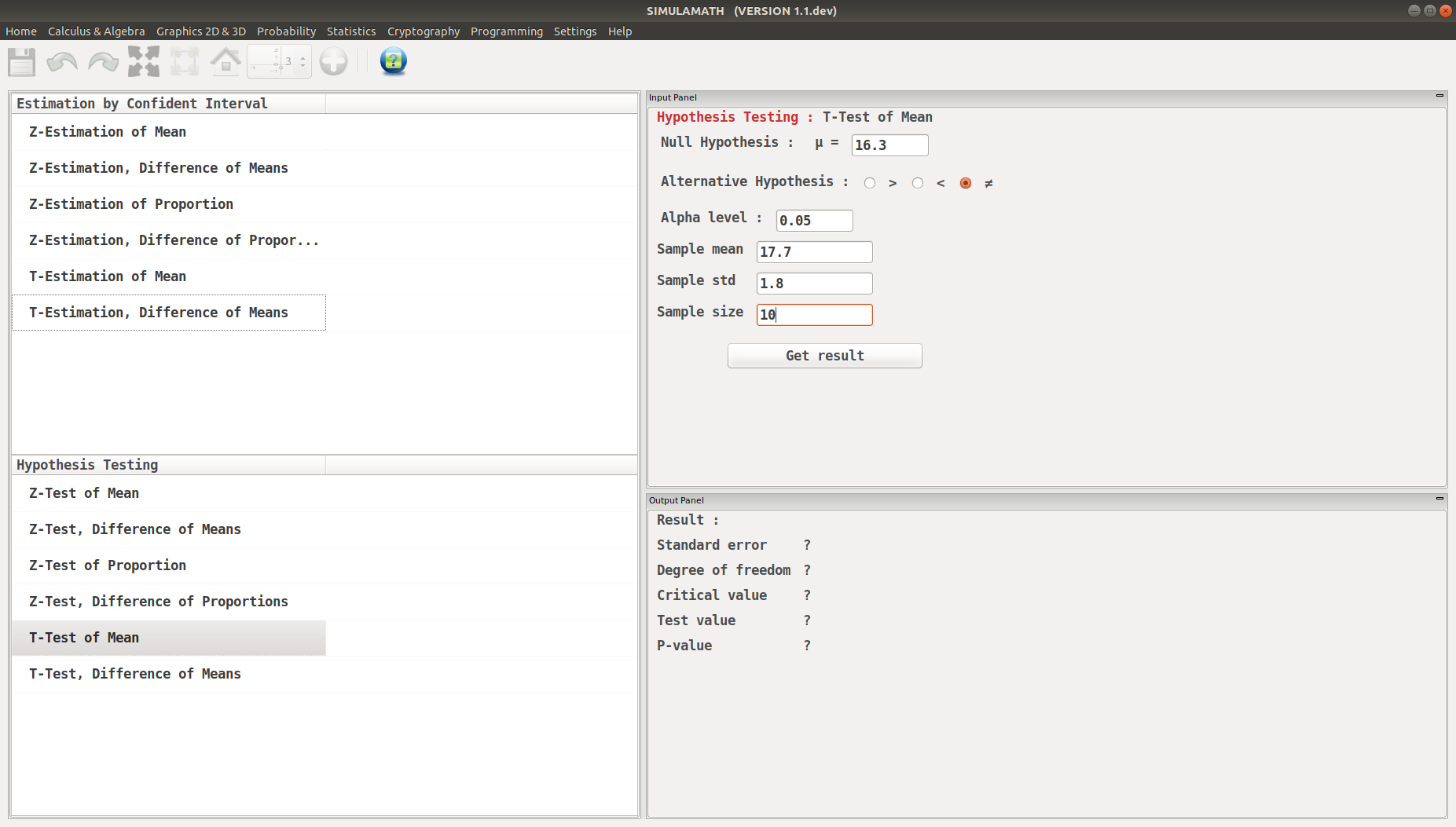
Enter the variables (Null Hypothesis, Alternative Hypothesis, Alpha value, Sample mean, Standard deviation of the population, Sample size) in the top panel on the right hand side.

Click on Get result located below inside the same panel. Voila, you have your results in the panel down on the right hand side.

T-Test, Difference of Means¶

The formula for hypothesis testing for T-Test, Difference of Means is:

\[t = \dfrac{(\bar{X_1}-\bar{X_2}) - (\mu_1-\mu_1)}{\sqrt{\dfrac{s_1^2}{n_1} + \dfrac{s_2^2}{n_2} }}\]

This formula is based on the general format of

\[\text{Test value} = \dfrac{(\text{observed value)} - (\text{expected value})} {\text{standard error}}\]

Assumptions for the t-Test for two independent Means when $\sigma_1$ and $\sigma_2$ are unknown

The samples are random samples.
The sample data are independent of one another.
When the sample sizes are less than 30, the populations must be normally or approximately normally distributed.

Example:

The average size of a farm in Indiana County, Pennsylvania, is 191 acres. The average size of a farm in Greene County, Pennsylvania, is 199 acres. Assume the data were obtained from two samples with standard deviations of 38 and 12 acres, respectively, and sample sizes of 8 and 10, respectively. Can it be concluded at $\alpha=0.05$ that the average size of the farms in the two counties is different? Assume the populations are normally distributed.

Solution:

Etape 1: State the hypotheses and identify the claim for the means.

\[H_0: \mu_1 = \mu_2 \quad \text{and} \quad H_1: \mu_1 \neq \mu_2 \quad \text{(claim)}\]

Etape 2: Find the critical values. Since the test is two-tailed, since $\alpha=0.05$, and since the variances are unequal, the degrees of freedom are the smaller of $n_1 - 1$ or $n2 - 1$. In this case, the degrees of freedom are $8 - 1 = 7$. Hence, from Table F, the critical values are +2.365 and -2.365.

Etape 3: Compute the test value. Since the variances are unequal, use the first formula.

\[t = \dfrac{(\bar{X_1}-\bar{X_2}) - (\mu_1-\mu_1)}{\sqrt{\dfrac{s_1^2}{n_1} + \dfrac{s_2^2}{n_2} }}\]

\[t = \dfrac{(191 - 199) - 0}{\sqrt{\dfrac{38^2}{8} + \dfrac{12^2}{10} }} = - 0.57\]

Stape 4: Make the decision. Do not reject the null hypothesis, since $-0.57 > -2.365$

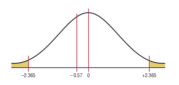
Stape 5: Summarize the results. There is not enough evidence to support the claim that the average size of the farms is different.

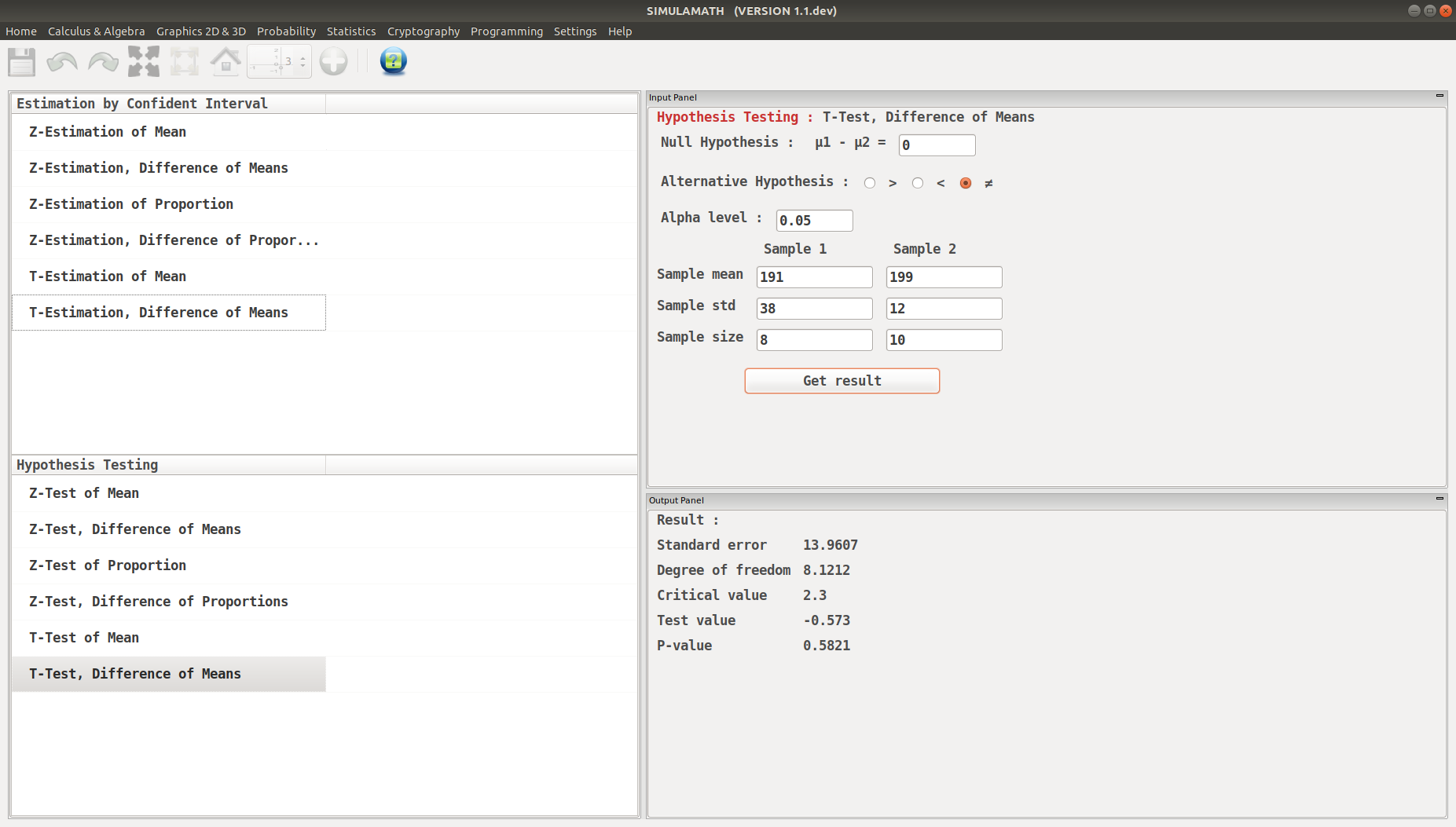
T-Test, Difference of Means in Simulamath¶

Choose the type of test/estimation you want to compute in the panels on the left hand side, here T-Estimation, Difference of Means

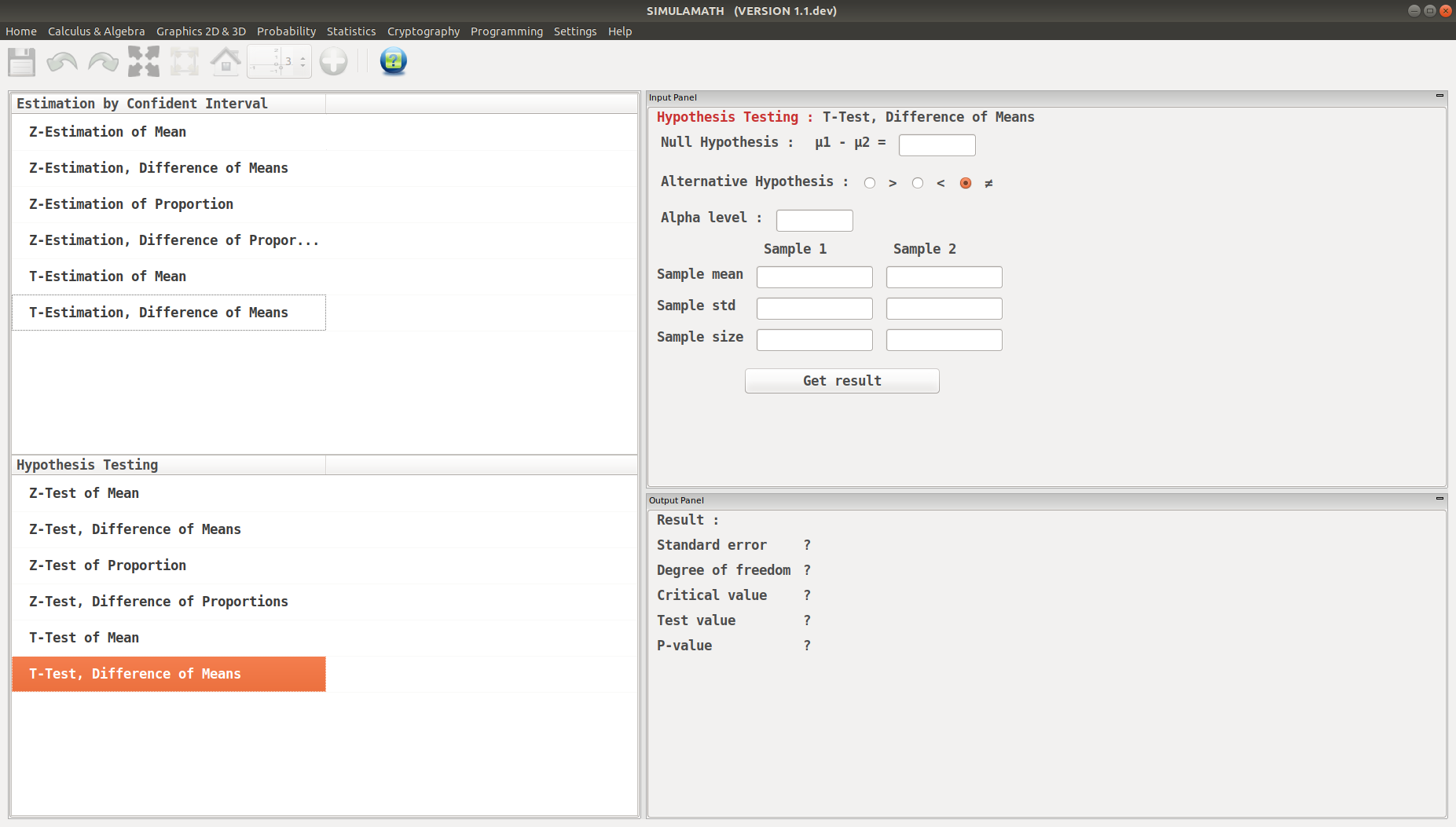
Enter the variables (Null Hypothesis, Alternative Hypothesis, Alpha value, Sample mean, Standard deviation of the population, Sample size) for each sample in the top panel on the right hand side.

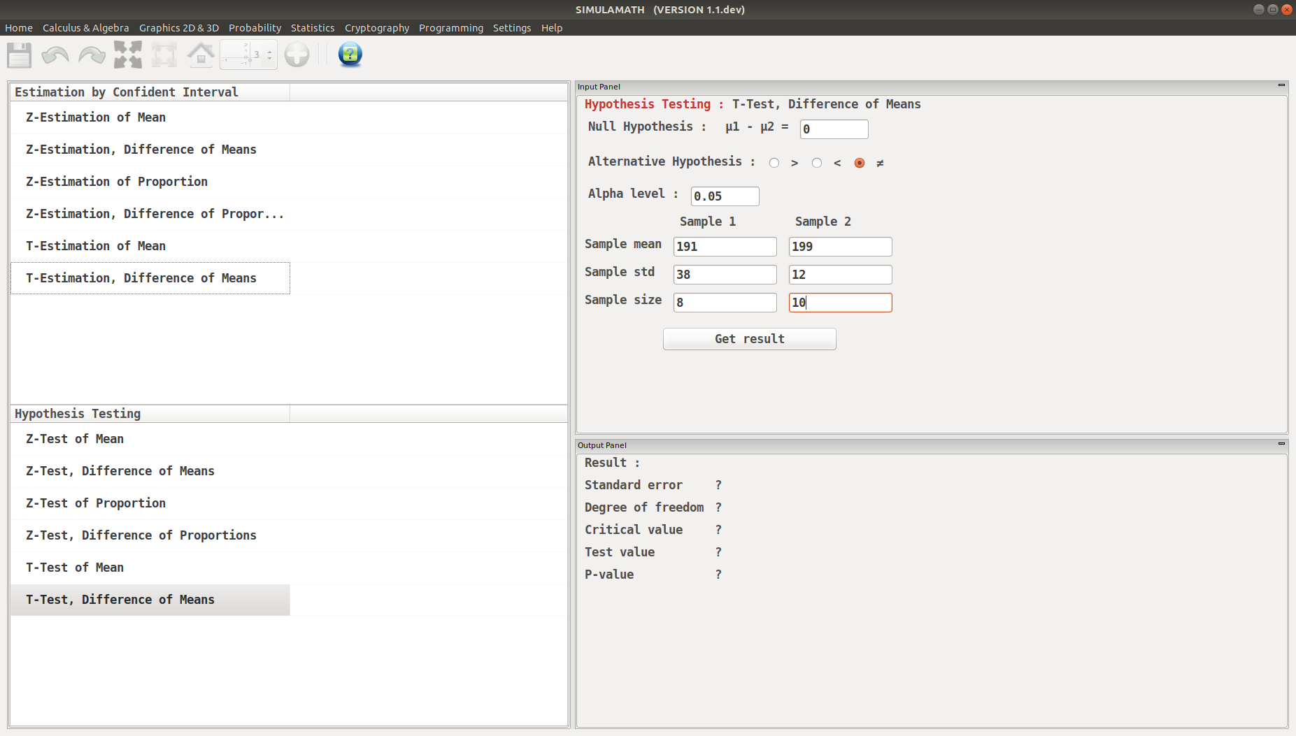
Click on Get result located below inside the same panel. Voila, you have your results in the panel down on the right hand side.